Archive for the ‘Business Intelligence’ Category
A gentle introduction to cluster analysis using R
Introduction
Welcome to the second part of my introductory series on text analysis using R (the first article can be accessed here). My aim in the present piece is to provide a practical introduction to cluster analysis. I’ll begin with some background before moving on to the nuts and bolts of clustering. We have a fair bit to cover, so let’s get right to it.
A common problem when analysing large collections of documents is to categorize them in some meaningful way. This is easy enough if one has a predefined classification scheme that is known to fit the collection (and if the collection is small enough to be browsed manually). One can then simply scan the documents, looking for keywords appropriate to each category and classify the documents based on the results. More often than not, however, such a classification scheme is not available and the collection too large. One then needs to use algorithms that can classify documents automatically based on their structure and content.
The present post is a practical introduction to a couple of automatic text categorization techniques, often referred to as clustering algorithms. As the Wikipedia article on clustering tells us:
Cluster analysis or clustering is the task of grouping a set of objects in such a way that objects in the same group (called a cluster) are more similar (in some sense or another) to each other than to those in other groups (clusters).
As one might guess from the above, the results of clustering depend rather critically on the method one uses to group objects. Again, quoting from the Wikipedia piece:
Cluster analysis itself is not one specific algorithm, but the general task to be solved. It can be achieved by various algorithms that differ significantly in their notion of what constitutes a cluster and how to efficiently find them. Popular notions of clusters include groups with small distances [Note: we’ll use distance-based methods] among the cluster members, dense areas of the data space, intervals or particular statistical distributions [i.e. distributions of words within documents and the entire collection].
…and a bit later:
…the notion of a “cluster” cannot be precisely defined, which is one of the reasons why there are so many clustering algorithms. There is a common denominator: a group of data objects. However, different researchers employ different cluster models, and for each of these cluster models again different algorithms can be given. The notion of a cluster, as found by different algorithms, varies significantly in its properties. Understanding these “cluster models” is key to understanding the differences between the various algorithms.
An upshot of the above is that it is not always straightforward to interpret the output of clustering algorithms. Indeed, we will see this in the example discussed below.
With that said for an introduction, let’s move on to the nut and bolts of clustering.
Preprocessing the corpus
In this section I cover the steps required to create the R objects necessary in order to do clustering. It goes over territory that I’ve covered in detail in the first article in this series – albeit with a few tweaks, so you may want to skim through even if you’ve read my previous piece.
To begin with I’ll assume you have R and RStudio (a free development environment for R) installed on your computer and are familiar with the basic functionality in the text mining ™ package. If you need help with this, please look at the instructions in my previous article on text mining.
As in the first part of this series, I will use 30 posts from my blog as the example collection (or corpus, in text mining-speak). The corpus can be downloaded here. For completeness, I will run through the entire sequence of steps – right from loading the corpus into R, to running the two clustering algorithms.
Ready? Let’s go…
The first step is to fire up RStudio and navigate to the directory in which you have unpacked the example corpus. Once this is done, load the text mining package, tm. Here’s the relevant code (Note: a complete listing of the code in this article can be accessed here):
[1] “C:/Users/Kailash/Documents”
#set working directory – fix path as needed!
setwd(“C:/Users/Kailash/Documents/TextMining”)
#load tm library
library(tm)
Loading required package: NLP
Note: R commands are in blue, output in black or red; lines that start with # are comments.
If you get an error here, you probably need to download and install the tm package. You can do this in RStudio by going to Tools > Install Packages and entering “tm”. When installing a new package, R automatically checks for and installs any dependent packages.
The next step is to load the collection of documents into an object that can be manipulated by functions in the tm package.
docs <- Corpus(DirSource("C:/Users/Kailash/Documents/TextMining"))
#inspect a particular document
writeLines(as.character(docs[[30]]))
…
The next step is to clean up the corpus. This includes things such as transforming to a consistent case, removing non-standard symbols & punctuation, and removing numbers (assuming that numbers do not contain useful information, which is the case here):
docs <- tm_map(docs,content_transformer(tolower))
#remove potentiallyy problematic symbols
toSpace <- content_transformer(function(x, pattern) { return (gsub(pattern, " ", x))})
docs <- tm_map(docs, toSpace, "-")
docs <- tm_map(docs, toSpace, ":")
docs <- tm_map(docs, toSpace, "‘")
docs <- tm_map(docs, toSpace, "•")
docs <- tm_map(docs, toSpace, "• ")
docs <- tm_map(docs, toSpace, " -")
docs <- tm_map(docs, toSpace, "“")
docs <- tm_map(docs, toSpace, "”")
#remove punctuation
docs <- tm_map(docs, removePunctuation)
#Strip digits
docs <- tm_map(docs, removeNumbers)
Note: please see my previous article for more on content_transformer and the toSpace function defined above.
Next we remove stopwords – common words (like “a” “and” “the”, for example) and eliminate extraneous whitespaces.
docs <- tm_map(docs, removeWords, stopwords("english"))
#remove whitespace
docs <- tm_map(docs, stripWhitespace)
writeLines(as.character(docs[[30]]))
flexibility eye beholder action increase organisational flexibility say redeploying employees likely seen affected move constrains individual flexibility dual meaning characteristic many organizational platitudes excellence synergy andgovernance interesting exercise analyse platitudes expose difference espoused actual meanings sign wishing many hours platitude deconstructing fun
At this point it is critical to inspect the corpus because stopword removal in tm can be flaky. Yes, this is annoying but not a showstopper because one can remove problematic words manually once one has identified them – more about this in a minute.
Next, we stem the document – i.e. truncate words to their base form. For example, “education”, “educate” and “educative” are stemmed to “educat.”:
Stemming works well enough, but there are some fixes that need to be done due to my inconsistent use of British/Aussie and US English. Also, we’ll take this opportunity to fix up some concatenations like “andgovernance” (see paragraph printed out above). Here’s the code:
docs <- tm_map(docs, content_transformer(gsub), pattern = "organis", replacement = "organ")
docs <- tm_map(docs, content_transformer(gsub), pattern = "andgovern", replacement = "govern")
docs <- tm_map(docs, content_transformer(gsub), pattern = "inenterpris", replacement = "enterpris")
docs <- tm_map(docs, content_transformer(gsub), pattern = "team-", replacement = "team")
The next step is to remove the stopwords that were missed by R. The best way to do this for a small corpus is to go through it and compile a list of words to be eliminated. One can then create a custom vector containing words to be removed and use the removeWords transformation to do the needful. Here is the code (Note: + indicates a continuation of a statement from the previous line):
+ "also","howev","tell","will",
+ "much","need","take","tend","even",
+ "like","particular","rather","said",
+ "get","well","make","ask","come","end",
+ "first","two","help","often","may",
+ "might","see","someth","thing","point",
+ "post","look","right","now","think","’ve ",
+ "’re ")
#remove custom stopwords
docs <- tm_map(docs, removeWords, myStopwords)
Again, it is a good idea to check that the offending words have really been eliminated.
The final preprocessing step is to create a document-term matrix (DTM) – a matrix that lists all occurrences of words in the corpus. In a DTM, documents are represented by rows and the terms (or words) by columns. If a word occurs in a particular document n times, then the matrix entry for corresponding to that row and column is n, if it doesn’t occur at all, the entry is 0.
Creating a DTM is straightforward– one simply uses the built-in DocumentTermMatrix function provided by the tm package like so:
#print a summary
dtmNon-/sparse entries: 13312/110618
Sparsity : 89%
Maximal term length: 48
Weighting : term frequency (tf)
This brings us to the end of the preprocessing phase. Next, I’ll briefly explain how distance-based algorithms work before going on to the actual work of clustering.
An intuitive introduction to the algorithms
As mentioned in the introduction, the basic idea behind document or text clustering is to categorise documents into groups based on likeness. Let’s take a brief look at how the algorithms work their magic.
Consider the structure of the DTM. Very briefly, it is a matrix in which the documents are represented as rows and words as columns. In our case, the corpus has 30 documents and 4131 words, so the DTM is a 30 x 4131 matrix. Mathematically, one can think of this matrix as describing a 4131 dimensional space in which each of the words represents a coordinate axis and each document is represented as a point in this space. This is hard to visualise of course, so it may help to illustrate this via a two-document corpus with only three words in total.
Consider the following corpus:
Document A: “five plus five”
Document B: “five plus six”
These two documents can be represented as points in a 3 dimensional space that has the words “five” “plus” and “six” as the three coordinate axes (see figure 1).
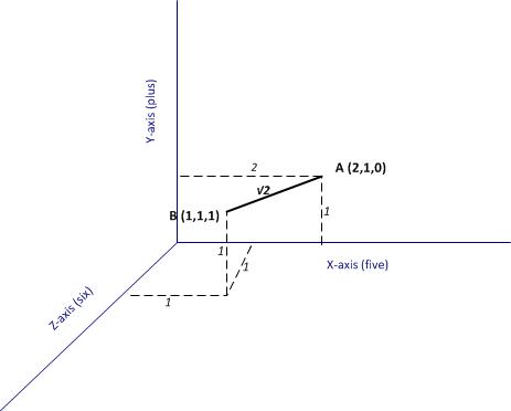
Figure 1: Documents A and B as points in a 3-word space
Now, if each of the documents can be thought of as a point in a space, it is easy enough to take the next logical step which is to define the notion of a distance between two points (i.e. two documents). In figure 1 the distance between A and B (which I denote as 

Generalising the above to the 4131 dimensional space at hand, the distance between two documents (let’s call them X and Y) have coordinates (word frequencies) 


It should be noted that the Euclidean distance that I have described is above is not the only possible way to define distance mathematically. There are many others but it would take me too far afield to discuss them here – see this article for more (and don’t be put off by the term metric, a metric in this context is merely a distance)
What’s important here is the idea that one can define a numerical distance between documents. Once this is grasped, it is easy to understand the basic idea behind how (some) clustering algorithms work – they group documents based on distance-related criteria. To be sure, this explanation is simplistic and glosses over some of the complicated details in the algorithms. Nevertheless it is a reasonable, approximate explanation for what goes on under the hood. I hope purists reading this will agree!
Finally, for completeness I should mention that there are many clustering algorithms out there, and not all of them are distance-based.
Hierarchical clustering
The first algorithm we’ll look at is hierarchical clustering. As the Wikipedia article on the topic tells us, strategies for hierarchical clustering fall into two types:
Agglomerative: where we start out with each document in its own cluster. The algorithm iteratively merges documents or clusters that are closest to each other until the entire corpus forms a single cluster. Each merge happens at a different (increasing) distance.
Divisive: where we start out with the entire set of documents in a single cluster. At each step the algorithm splits the cluster recursively until each document is in its own cluster. This is basically the inverse of an agglomerative strategy.
The algorithm we’ll use is hclust which does agglomerative hierarchical clustering. Here’s a simplified description of how it works:
- Assign each document to its own (single member) cluster
- Find the pair of clusters that are closest to each other and merge them. So you now have one cluster less than before.
- Compute distances between the new cluster and each of the old clusters.
- Repeat steps 2 and 3 until you have a single cluster containing all documents.
We’ll need to do a few things before running the algorithm. Firstly, we need to convert the DTM into a standard matrix which can be used by dist, the distance computation function in R (the DTM is not stored as a standard matrix). We’ll also shorten the document names so that they display nicely in the graph that we will use to display results of hclust (the names I have given the documents are just way too long). Here’s the relevant code:
m <- as.matrix(dtm)
#write as csv file (optional)
write.csv(m,file="dtmEight2Late.csv")
#shorten rownames for display purposes
rownames(m) <- paste(substring(rownames(m),1,3),rep("..",nrow(m)),
+ substring(rownames(m), nchar(rownames(m))-12,nchar(rownames(m))-4))
#compute distance between document vectors
d <- dist(m)
Next we run hclust. The algorithm offers several options check out the documentation for details. I use a popular option called Ward’s method – there are others, and I suggest you experiment with them as each of them gives slightly different results making interpretation somewhat tricky (did I mention that clustering is as much an art as a science??). Finally, we visualise the results in a dendogram (see Figure 2 below).
#run hierarchical clustering using Ward’s method
groups <- hclust(d,method="ward.D")
#plot dendogram, use hang to ensure that labels fall below tree
plot(groups, hang=-1)

Figure 2: Dendogram from hierarchical clustering of corpus
A few words on interpreting dendrograms for hierarchical clusters: as you work your way down the tree in figure 2, each branch point you encounter is the distance at which a cluster merge occurred. Clearly, the most well-defined clusters are those that have the largest separation; many closely spaced branch points indicate a lack of dissimilarity (i.e. distance, in this case) between clusters. Based on this, the figure reveals that there are 2 well-defined clusters – the first one consisting of the three documents at the right end of the cluster and the second containing all other documents. We can display the clusters on the graph using the rect.hclust function like so:
rect.hclust(groups,2)
The result is shown in the figure below.

Figure 3: 2 cluster grouping
The figures 4 and 5 below show the grouping for 3, and 5 clusters.

Figure 4: 3 cluster grouping
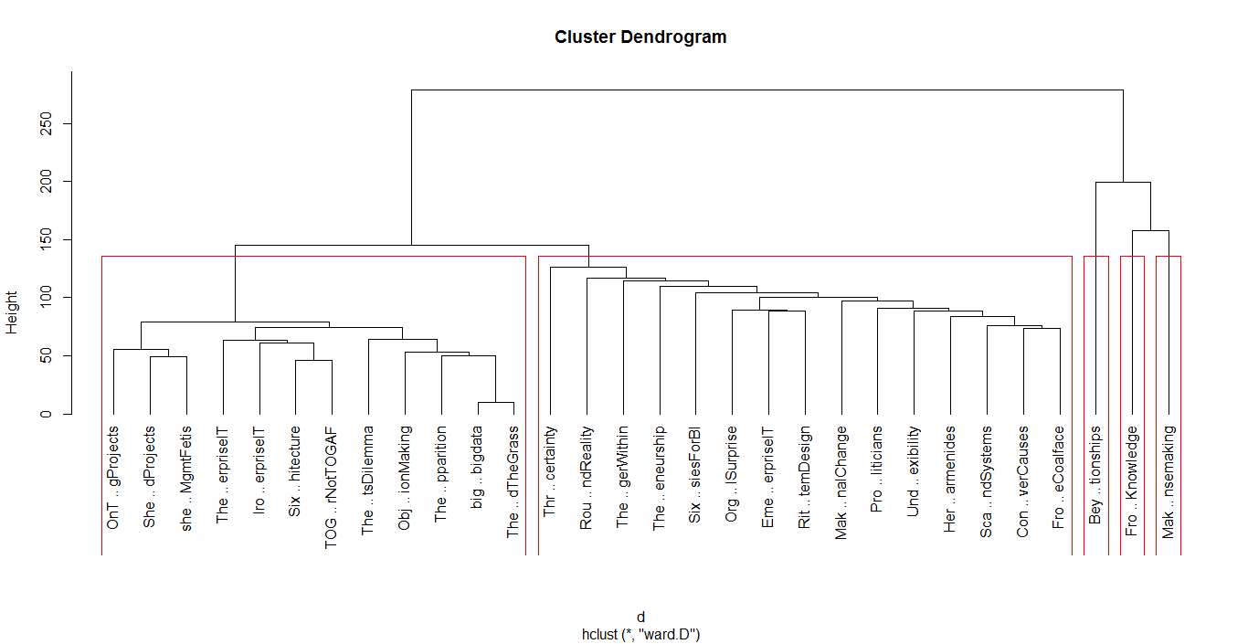
Figure 5: 5 cluster grouping
I’ll make just one point here: the 2 cluster grouping seems the most robust one as it happens at large distance, and is cleanly separated (distance-wise) from the 3 and 5 cluster grouping. That said, I’ll leave you to explore the ins and outs of hclust on your own and move on to our next algorithm.
K means clustering
In hierarchical clustering we did not specify the number of clusters upfront. These were determined by looking at the dendogram after the algorithm had done its work. In contrast, our next algorithm – K means – requires us to define the number of clusters upfront (this number being the “k” in the name). The algorithm then generates k document clusters in a way that ensures the within-cluster distances from each cluster member to the centroid (or geometric mean) of the cluster is minimised.
Here’s a simplified description of the algorithm:
- Assign the documents randomly to k bins
- Compute the location of the centroid of each bin.
- Compute the distance between each document and each centroid
- Assign each document to the bin corresponding to the centroid closest to it.
- Stop if no document is moved to a new bin, else go to step 2.
An important limitation of the k means method is that the solution found by the algorithm corresponds to a local rather than global minimum (this figure from Wikipedia explains the difference between the two in a nice succinct way). As a consequence it is important to run the algorithm a number of times (each time with a different starting configuration) and then select the result that gives the overall lowest sum of within-cluster distances for all documents. A simple check that a solution is robust is to run the algorithm for an increasing number of initial configurations until the result does not change significantly. That said, this procedure does not guarantee a globally optimal solution.
I reckon that’s enough said about the algorithm, let’s get on with it using it. The relevant function, as you might well have guessed is kmeans. As always, I urge you to check the documentation to understand the available options. We’ll use the default options for all parameters excepting nstart which we set to 100. We also plot the result using the clusplot function from the cluster library (which you may need to install. Reminder you can install packages via the Tools>Install Packages menu in RStudio)
kfit <- kmeans(d, 2, nstart=100)
#plot – need library cluster
library(cluster)
clusplot(as.matrix(d), kfit$cluster, color=T, shade=T, labels=2, lines=0)
The plot is shown in Figure 6.
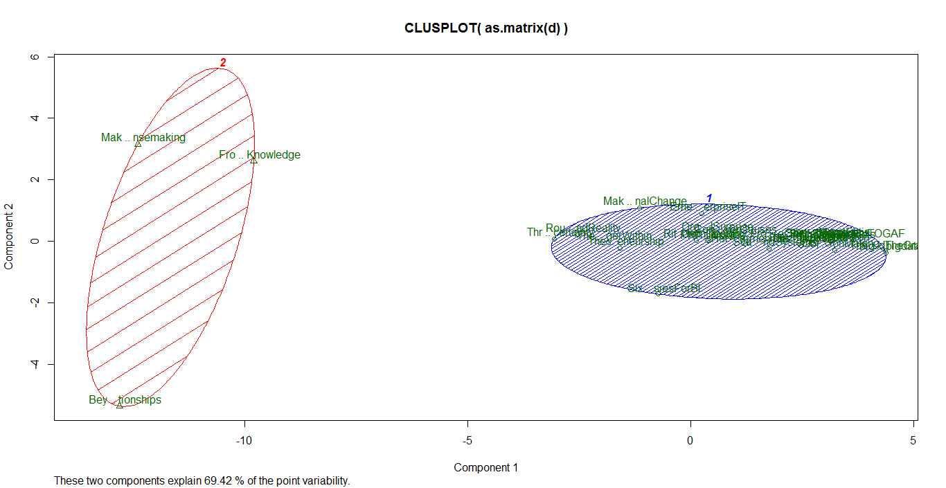
Figure 6: principal component plot (k=2)
The cluster plot shown in the figure above needs a bit of explanation. As mentioned earlier, the clustering algorithms work in a mathematical space whose dimensionality equals the number of words in the corpus (4131 in our case). Clearly, this is impossible to visualize. To handle this, mathematicians have invented a dimensionality reduction technique called Principal Component Analysis which reduces the number of dimensions to 2 (in this case) in such a way that the reduced dimensions capture as much of the variability between the clusters as possible (and hence the comment, “these two components explain 69.42% of the point variability” at the bottom of the plot in figure 6)
(Aside Yes I realize the figures are hard to read because of the overly long names, I leave it to you to fix that. No excuses, you know how…:-))
Running the algorithm and plotting the results for k=3 and 5 yields the figures below.

Figure 7: Principal component plot (k=3)

Figure 8: Principal component plot (k=5)
Choosing k
Recall that the k means algorithm requires us to specify k upfront. A natural question then is: what is the best choice of k? In truth there is no one-size-fits-all answer to this question, but there are some heuristics that might sometimes help guide the choice. For completeness I’ll describe one below even though it is not much help in our clustering problem.
In my simplified description of the k means algorithm I mentioned that the technique attempts to minimise the sum of the distances between the points in a cluster and the cluster’s centroid. Actually, the quantity that is minimised is the total of the within-cluster sum of squares (WSS) between each point and the mean. Intuitively one might expect this quantity to be maximum when k=1 and then decrease as k increases, sharply at first and then less sharply as k reaches its optimal value.
The problem with this reasoning is that it often happens that the within cluster sum of squares never shows a slowing down in decrease of the summed WSS. Unfortunately this is exactly what happens in the case at hand.
I reckon a picture might help make the above clearer. Below is the R code to draw a plot of summed WSS as a function of k for k=2 all the way to 29 (1-total number of documents):
#look for “elbow” in plot of summed intra-cluster distances (withinss) as fn of k
wss <- 2:29
for (i in 2:29) wss[i] <- sum(kmeans(d,centers=i,nstart=25)$withinss)
plot(2:29, wss[2:29], type="b", xlab="Number of Clusters",ylab="Within groups sum of squares")
…and the figure below shows the resulting plot.

Figure 10: WSS as a function of k (“elbow plot”)
The plot clearly shows that there is no k for which the summed WSS flattens out (no distinct “elbow”). As a result this method does not help. Fortunately, in this case one can get a sensible answer using common sense rather than computation: a choice of 2 clusters seems optimal because both algorithms yield exactly the same clusters and show the clearest cluster separation at this point (review the dendogram and cluster plots for k=2).
The meaning of it all
Now I must acknowledge an elephant in the room that I have steadfastly ignored thus far. The odds are good that you’ve seen it already….
It is this: what topics or themes do the (two) clusters correspond to?
Unfortunately this question does not have a straightforward answer. Although the algorithms suggest a 2-cluster grouping, they are silent on the topics or themes related to these. Moreover, as you will see if you experiment, the results of clustering depend on:
- The criteria for the construction of the DTM (see the documentation for DocumentTermMatrix for options).
- The clustering algorithm itself.
Indeed, insofar as clustering is concerned, subject matter and corpus knowledge is the best way to figure out cluster themes. This serves to reinforce (yet again!) that clustering is as much an art as it is a science.
In the case at hand, article length seems to be an important differentiator between the 2 clusters found by both algorithms. The three articles in the smaller cluster are in the top 4 longest pieces in the corpus. Additionally, the three pieces are related to sensemaking and dialogue mapping. There are probably other factors as well, but none that stand out as being significant. I should mention, however, that the fact that article length seems to play a significant role here suggests that it may be worth checking out the effect of scaling distances by word counts or using other measures such a cosine similarity – but that’s a topic for another post! (Note added on Dec 3 2015: check out my article on visualizing relationships between documents using network graphs for a detailed discussion on cosine similarity)
The take home lesson is that is that the results of clustering are often hard to interpret. This should not be surprising – the algorithms cannot interpret meaning, they simply chug through a mathematical optimisation problem. The onus is on the analyst to figure out what it means…or if it means anything at all.
Conclusion
This brings us to the end of a long ramble through clustering. We’ve explored the two most common methods: hierarchical and k means clustering (there are many others available in R, and I urge you to explore them). Apart from providing the detailed steps to do clustering, I have attempted to provide an intuitive explanation of how the algorithms work. I hope I have succeeded in doing so. As always your feedback would be very welcome.
Finally, I’d like to reiterate an important point: the results of our clustering exercise do not have a straightforward interpretation, and this is often the case in cluster analysis. Fortunately I can close on an optimistic note. There are other text mining techniques that do a better job in grouping documents based on topics and themes rather than word frequencies alone. I’ll discuss this in the next article in this series. Until then, I wish you many enjoyable hours exploring the ins and outs of clustering.
Note added on September 29th 2015:
If you liked this article, you might want to check out its sequel – an introduction to topic modeling.
A gentle introduction to text mining using R
Preamble
This article is based on my exploration of the basic text mining capabilities of R, the open source statistical software. It is intended primarily as a tutorial for novices in text mining as well as R. However, unlike conventional tutorials, I spend a good bit of time setting the context by describing the problem that led me to text mining and thence to R. I also talk about the limitations of the techniques I describe, and point out directions for further exploration for those who are interested. Indeed, I’ll likely explore some of these myself in future articles.
If you have no time and /or wish to cut to the chase, please go straight to the section entitled, Preliminaries – installing R and RStudio. If you have already installed R and have worked with it, you may want to stop reading as I doubt there’s anything I can tell you that you don’t already know 🙂
A couple of warnings are in order before we proceed. R and the text mining options we explore below are open source software. Version differences in open source can be significant and are not always documented in a way that corporate IT types are used to. Indeed, I was tripped up by such differences in an earlier version of this article (now revised). So, just for the record, the examples below were run on version 3.2.0 of R and version 0.6-1 of the tm (text mining) package for R. A second point follows from this: as is evident from its version number, the tm package is still in the early stages of its evolution. As a result – and we will see this below – things do not always work as advertised. So assume nothing, and inspect the results in detail at every step. Be warned that I do not always do this below, as my aim is introduction rather than accuracy.
Background and motivation
Traditional data analysis is based on the relational model in which data is stored in tables. Within tables, data is stored in rows – each row representing a single record of an entity of interest (such as a customer or an account). The columns represent attributes of the entity. For example, the customer table might consist of columns such as name, street address, city, postcode, telephone number . Typically these are defined upfront, when the data model is created. It is possible to add columns after the fact, but this tends to be messy because one also has to update existing rows with information pertaining to the added attribute.
As long as one asks for information that is based only on existing attributes – an example being, “give me a list of customers based in Sydney” – a database analyst can use Structured Query Language (the defacto language of relational databases ) to get an answer. A problem arises, however, if one asks for information that is based on attributes that are not included in the database. An example in the above case would be: “give me a list of customers who have made a complaint in the last twelve months.”
As a result of the above, many data modelers will include a “catch-all” free text column that can be used to capture additional information in an ad-hoc way. As one might imagine, this column will often end up containing several lines, or even paragraphs of text that are near impossible to analyse with the tools available in relational databases.
(Note: for completeness I should add that most database vendors have incorporated text mining capabilities into their products. Indeed, many of them now include R…which is another good reason to learn it.)
My story
Over the last few months, when time permits, I’ve been doing an in-depth exploration of the data captured by my organisation’s IT service management tool. Such tools capture all support tickets that are logged, and track their progress until they are closed. As it turns out, there are a number of cases where calls are logged against categories that are too broad to be useful – the infamous catch-all category called “Unknown.” In such cases, much of the important information is captured in a free text column, which is difficult to analyse unless one knows what one is looking for. The problem I was grappling with was to identify patterns and hence define sub-categories that would enable support staff to categorise these calls meaningfully.
One way to do this is to guess what the sub-categories might be…and one can sometimes make pretty good guesses if one knows the data well enough. In general, however, guessing is a terrible strategy because one does not know what one does not know. The only sensible way to extract subcategories is to analyse the content of the free text column systematically. This is a classic text mining problem.
Now, I knew a bit about the theory of text mining, but had little practical experience with it. So the logical place for me to start was to look for a suitable text mining tool. Our vendor (who shall remain unnamed) has a “Rolls-Royce” statistical tool that has a good text mining add-on. We don’t have licenses for the tool, but the vendor was willing to give us a trial license for a few months…with the understanding that this was on an intent-to-purchase basis.
I therefore started looking at open source options. While doing so, I stumbled on an interesting paper by Ingo Feinerer that describes a text mining framework for the R environment. Now, I knew about R, and was vaguely aware that it offered text mining capabilities, but I’d not looked into the details. Anyway, I started reading the paper…and kept going until I finished.
As I read, I realised that this could be the answer to my problems. Even better, it would not require me trade in assorted limbs for a license.
I decided to give it a go.
Preliminaries – installing R and RStudio
R can be downloaded from the R Project website. There is a Windows version available, which installed painlessly on my laptop. Commonly encountered installation issues are answered in the (very helpful) R for Windows FAQ.
RStudio is an integrated development environment (IDE) for R. There is a commercial version of the product, but there is also a free open source version. In what follows, I’ve used the free version. Like R, RStudio installs painlessly and also detects your R installation.
RStudio has the following panels:
- A script editor in which you can create R scripts (top left). You can also open a new script editor window by going to File > New File > RScript.
- The console where you can execute R commands/scripts (bottom left)
- Environment and history (top right)
- Files in the current working directory, installed R packages, plots and a help display screen (bottom right).
Check out this short video for a quick introduction to RStudio.
You can access help anytime (within both R and RStudio) by typing a question mark before a command. Exercise: try this by typing ?getwd() and ?setwd() in the console.
I should reiterate that the installation process for both products was seriously simple…and seriously impressive. “Rolls-Royce” business intelligence vendors could take a lesson from that…in addition to taking a long hard look at the ridiculous prices they charge.
There is another small step before we move on to the fun stuff. Text mining and certain plotting packages are not installed by default so one has to install them manually The relevant packages are:
- tm – the text mining package (see documentation). Also check out this excellent introductory article on tm.
- SnowballC – required for stemming (explained below).
- ggplot2 – plotting capabilities (see documentation)
- wordcloud – which is self-explanatory (see documentation) .
(Warning for Windows users: R is case-sensitive so Wordcloud != wordcloud)
The simplest way to install packages is to use RStudio’s built in capabilities (go to Tools > Install Packages in the menu). If you’re working on Windows 7 or 8, you might run into a permissions issue when installing packages. If you do, you might find this advice from the R for Windows FAQ helpful.
Preliminaries – The example dataset
The data I had from our service management tool isn’t the best dataset to learn with as it is quite messy. But then, I have a reasonable data source in my virtual backyard: this blog. To this end, I converted all posts I’ve written since Dec 2013 into plain text form (30 posts in all). You can download the zip file of these here .
I suggest you create a new folder called – called, say, TextMining – and unzip the files in that folder.
That done, we’re good to start…
Preliminaries – Basic Navigation
A few things to note before we proceed:
- In what follows, I enter the commands directly in the console. However, here’s a little RStudio tip that you may want to consider: you can enter an R command or code fragment in the script editor and then hit Ctrl-Enter (i.e. hit the Enter key while holding down the Control key) to copy the line to the console. This will enable you to save the script as you go along.
- In the code snippets below, the functions / commands to be typed in the R console are in blue font. The output is in black. I will also denote references to functions / commands in the body of the article by italicising them as in “setwd()”. Be aware that I’ve omitted the command prompt “>” in the code snippets below!
- It is best not to cut-n-paste commands directly from the article as quotes are sometimes not rendered correctly. A text file of all the code in this article is available here.
The > prompt in the RStudio console indicates that R is ready to process commands.
To see the current working directory type in getwd() and hit return. You’ll see something like:
[1] “C:/Users/Documents”
The exact output will of course depend on your working directory. Note the forward slashes in the path. This is because of R’s Unix heritage (backslash is an escape character in R.). So, here’s how would change the working directory to C:\Users:
You can now use getwd()to check that setwd() has done what it should.
[1]”C:/Users”
I won’t say much more here about R as I want to get on with the main business of the article. Check out this very short introduction to R for a quick crash course.
Loading data into R
Start RStudio and open the TextMining project you created earlier.
The next step is to load the tm package as this is not loaded by default. This is done using the library() function like so:
Dependent packages are loaded automatically – in this case the dependency is on the NLP (natural language processing) package.
Next, we need to create a collection of documents (technically referred to as a Corpus) in the R environment. This basically involves loading the files created in the TextMining folder into a Corpus object. The tm package provides the Corpus() function to do this. There are several ways to create a Corpus (check out the online help using ? as explained earlier). In a nutshell, the Corpus() function can read from various sources including a directory. That’s the option we’ll use:
docs <- Corpus(DirSource(“C:/Users/Kailash/Documents/TextMining”))
At the risk of stating the obvious, you will need to tailor this path as appropriate.
A couple of things to note in the above. Any line that starts with a # is a comment, and the “<-“ tells R to assign the result of the command on the right hand side to the variable on the left hand side. In this case the Corpus object created is stored in a variable called docs. One can also use the equals sign (=) for assignment if one wants to.
Type in docs to see some information about the newly created corpus:
Metadata: corpus specific: 0, document level (indexed): 0
Content: documents: 30
The summary() function gives more details, including a complete listing of files…but it isn’t particularly enlightening. Instead, we’ll examine a particular document in the corpus.
writeLines(as.character(docs[[30]]))
Which prints the entire content of 30th document in the corpus to the console.
Pre-processing
Data cleansing, though tedious, is perhaps the most important step in text analysis. As we will see, dirty data can play havoc with the results. Furthermore, as we will also see, data cleaning is invariably an iterative process as there are always problems that are overlooked the first time around.
The tm package offers a number of transformations that ease the tedium of cleaning data. To see the available transformations type getTransformations() at the R prompt:
> getTransformations()
[1] “removeNumbers” “removePunctuation” “removeWords” “stemDocument” “stripWhitespace”
Most of these are self-explanatory. I’ll explain those that aren’t as we go along.
There are a few preliminary clean-up steps we need to do before we use these powerful transformations. If you inspect some documents in the corpus (and you know how to do that now), you will notice that I have some quirks in my writing. For example, I often use colons and hyphens without spaces between the words separated by them. Using the removePunctuation transform without fixing this will cause the two words on either side of the symbols to be combined. Clearly, we need to fix this prior to using the transformations.
To fix the above, one has to create a custom transformation. The tm package provides the ability to do this via the content_transformer function. This function takes a function as input, the input function should specify what transformation needs to be done. In this case, the input function would be one that replaces all instances of a character by spaces. As it turns out the gsub() function does just that.
Here is the R code to build the content transformer, which we will call toSpace:
Now we can use this content transformer to eliminate colons and hypens like so:
docs <- tm_map(docs, toSpace, “:”)
Inspect random sections f corpus to check that the result is what you intend (use writeLines as shown earlier). To reiterate something I mentioned in the preamble, it is good practice to inspect the a subset of the corpus after each transformation.
If it all looks good, we can now apply the removePunctuation transformation. This is done as follows:
Inspecting the corpus reveals that several “non-standard” punctuation marks have not been removed. These include the single curly quote marks and a space-hyphen combination. These can be removed using our custom content transformer, toSpace. Note that you might want to copy-n-paste these symbols directly from the relevant text file to ensure that they are accurately represented in toSpace.
docs <- tm_map(docs, toSpace, “‘”)
docs <- tm_map(docs, toSpace, ” -“)
Inspect the corpus again to ensure that the offenders have been eliminated. This is also a good time to check for any other special symbols that may need to be removed manually.
If all is well, you can move to the next step which is to:
- Convert the corpus to lower case
- Remove all numbers.
Since R is case sensitive, “Text” is not equal to “text” – and hence the rationale for converting to a standard case. However, although there is a tolower transformation, it is not a part of the standard tm transformations (see the output of getTransformations() in the previous section). For this reason, we have to convert tolower into a transformation that can handle a corpus object properly. This is done with the help of our new friend, content_transformer.
Here’s the relevant code:
docs <- tm_map(docs,content_transformer(tolower))
Text analysts are typically not interested in numbers since these do not usually contribute to the meaning of the text. However, this may not always be so. For example, it is definitely not the case if one is interested in getting a count of the number of times a particular year appears in a corpus. This does not need to be wrapped in content_transformer as it is a standard transformation in tm.
docs <- tm_map(docs, removeNumbers)
Once again, be sure to inspect the corpus before proceeding.
The next step is to remove common words from the text. These include words such as articles (a, an, the), conjunctions (and, or but etc.), common verbs (is), qualifiers (yet, however etc) . The tm package includes a standard list of such stop words as they are referred to. We remove stop words using the standard removeWords transformation like so:
docs <- tm_map(docs, removeWords, stopwords(“english”))
Finally, we remove all extraneous whitespaces using the stripWhitespace transformation:
docs <- tm_map(docs, stripWhitespace)
Stemming
Typically a large corpus will contain many words that have a common root – for example: offer, offered and offering. Stemming is the process of reducing such related words to their common root, which in this case would be the word offer.
Simple stemming algorithms (such as the one in tm) are relatively crude: they work by chopping off the ends of words. This can cause problems: for example, the words mate and mating might be reduced to mat instead of mate. That said, the overall benefit gained from stemming more than makes up for the downside of such special cases.
To see what stemming does, let’s take a look at the last few lines of the corpus before and after stemming. Here’s what the last bit looks like prior to stemming (note that this may differ for you, depending on the ordering of the corpus source files in your directory):
flexibility eye beholder action increase organisational flexibility say redeploying employees likely seen affected move constrains individual flexibility dual meaning characteristic many organizational platitudes excellence synergy andgovernance interesting exercise analyse platitudes expose difference espoused actual meanings sign wishing many hours platitude deconstructing fun
Now let’s stem the corpus and reinspect it.
writeLines(as.character(docs[[30]]))
flexibl eye behold action increas organis flexibl say redeploy employe like seen affect move constrain individu flexibl dual mean characterist mani organiz platitud excel synergi andgovern interest exercis analys platitud expos differ espous actual mean sign wish mani hour platitud deconstruct fun
A careful comparison of the two paragraphs reveals the benefits and tradeoff of this relatively crude process.
There is a more sophisticated procedure called lemmatization that takes grammatical context into account. Among other things, determining the lemma of a word requires a knowledge of its part of speech (POS) – i.e. whether it is a noun, adjective etc. There are POS taggers that automate the process of tagging terms with their parts of speech. Although POS taggers are available for R (see this one, for example), I will not go into this topic here as it would make a long post even longer.
On another important note, the output of the corpus also shows up a problem or two. First, organiz and organis are actually variants of the same stem organ. Clearly, they should be merged. Second, the word andgovern should be separated out into and and govern (this is an error in the original text). These (and other errors of their ilk) can and should be fixed up before proceeding. This is easily done using gsub() wrapped in content_transformer. Here is the code to clean up these and a few other issues that I found:
Note that I have removed the stop words and and in in the 3rd and 4th transforms above.
There are definitely other errors that need to be cleaned up, but I’ll leave these for you to detect and remove.
The document term matrix
The next step in the process is the creation of the document term matrix (DTM)– a matrix that lists all occurrences of words in the corpus, by document. In the DTM, the documents are represented by rows and the terms (or words) by columns. If a word occurs in a particular document, then the matrix entry for corresponding to that row and column is 1, else it is 0 (multiple occurrences within a document are recorded – that is, if a word occurs twice in a document, it is recorded as “2” in the relevant matrix entry).
A simple example might serve to explain the structure of the TDM more clearly. Assume we have a simple corpus consisting of two documents, Doc1 and Doc2, with the following content:
Doc1: bananas are yellow
Doc2: bananas are good
The DTM for this corpus would look like:
| bananas | are | yellow | good | |
| Doc1 | 1 | 1 | 1 | 0 |
| Doc2 | 1 | 1 | 0 | 1 |
Clearly there is nothing special about rows and columns – we could just as easily transpose them. If we did so, we’d get a term document matrix (TDM) in which the terms are rows and documents columns. One can work with either a DTM or TDM. I’ll use the DTM in what follows.
There are a couple of general points worth making before we proceed. Firstly, DTMs (or TDMs) can be huge – the dimension of the matrix would be number of document x the number of words in the corpus. Secondly, it is clear that the large majority of words will appear only in a few documents. As a result a DTM is invariably sparse – that is, a large number of its entries are 0.
The business of creating a DTM (or TDM) in R is as simple as:
This creates a term document matrix from the corpus and stores the result in the variable dtm. One can get summary information on the matrix by typing the variable name in the console and hitting return:
<<DocumentTermMatrix (documents: 30, terms: 4209)>>
Non-/sparse entries: 14252/112018
Sparsity : 89%
Maximal term length: 48
Weighting : term frequency (tf)
This is a 30 x 4209 dimension matrix in which 89% of the rows are zero.
One can inspect the DTM, and you might want to do so for fun. However, it isn’t particularly illuminating because of the sheer volume of information that will flash up on the console. To limit the information displayed, one can inspect a small section of it like so:
<<DocumentTermMatrix (documents: 2, terms: 6)>>
Non-/sparse entries: 0/12
Sparsity : 100%
Maximal term length: 8
Weighting : term frequency (tf)
Docs creation creativ credibl credit crimin crinkl
BeyondEntitiesAndRelationships.txt 0 0 0 0 0 0
bigdata.txt 0 0 0 0 0 0
This command displays terms 1000 through 1005 in the first two rows of the DTM. Note that your results may differ.
Mining the corpus
Notice that in constructing the TDM, we have converted a corpus of text into a mathematical object that can be analysed using quantitative techniques of matrix algebra. It should be no surprise, therefore, that the TDM (or DTM) is the starting point for quantitative text analysis.
For example, to get the frequency of occurrence of each word in the corpus, we simply sum over all rows to give column sums:
Here we have first converted the TDM into a mathematical matrix using the as.matrix() function. We have then summed over all rows to give us the totals for each column (term). The result is stored in the (column matrix) variable freq.
Check that the dimension of freq equals the number of terms:
length(freq)
[1] 4209
Next, we sort freq in descending order of term count:
ord <- order(freq,decreasing=TRUE)
Then list the most and least frequently occurring terms:
freq[head(ord)]
one organ can manag work system
314 268 244 222 202 193
#inspect least frequently occurring terms
freq[tail(ord)]
yield yorkshir youtub zeno zero zulli
1 1 1 1 1 1
The least frequent terms can be more interesting than one might think. This is because terms that occur rarely are likely to be more descriptive of specific documents. Indeed, I can recall the posts in which I have referred to Yorkshire, Zeno’s Paradox and Mr. Lou Zulli without having to go back to the corpus, but I’d have a hard time enumerating the posts in which I’ve used the word system.
There are at least a couple of ways to simple ways to strike a balance between frequency and specificity. One way is to use so-called inverse document frequencies. A simpler approach is to eliminate words that occur in a large fraction of corpus documents. The latter addresses another issue that is evident in the above. We deal with this now.
Words like “can” and “one” give us no information about the subject matter of the documents in which they occur. They can therefore be eliminated without loss. Indeed, they ought to have been eliminated by the stopword removal we did earlier. However, since such words occur very frequently – virtually in all documents – we can remove them by enforcing bounds when creating the DTM, like so:
bounds = list(global = c(3,27))))
Here we have told R to include only those words that occur in 3 to 27 documents. We have also enforced lower and upper limit to length of the words included (between 4 and 20 characters).
Inspecting the new DTM:
<<DocumentTermMatrix (documents: 30, terms: 1290)>>
Non-/sparse entries: 10002/28698
Sparsity : 74%
Maximal term length: 15
Weighting : term frequency (tf)
The dimension is reduced to 30 x 1290.
Let’s calculate the cumulative frequencies of words across documents and sort as before:
#length should be total number of terms
length(freqr)
[1] 1290
#create sort order (asc)
ordr <- order(freqr,decreasing=TRUE)
#inspect most frequently occurring terms
freqr[head(ordr)]
organ manag work system project problem
268 222 202 193 184 171
#inspect least frequently occurring terms
freqr[tail(ordr)]
wait warehous welcom whiteboard wider widespread
3 3 3 3 3 3
The results make sense: the top 6 keywords are pretty good descriptors of what my blogs is about – projects, management and systems. However, not all high frequency words need be significant. What they do, is give you an idea of potential classification terms.
That done, let’s take get a list of terms that occur at least a 100 times in the entire corpus. This is easily done using the findFreqTerms() function as follows:
[1] “action” “approach” “base” “busi” “chang” “consult” “data” “decis” “design”
[10] “develop” “differ” “discuss” “enterpris” “exampl” “group” “howev” “import” “issu”
[19] “like” “make” “manag” “mani” “model” “often” “organ” “peopl” “point”
[28] “practic” “problem” “process” “project” “question” “said” “system” “thing” “think”
[37] “time” “understand” “view” “well” “will” “work”
Here I have asked findFreqTerms() to return all terms that occur more than 80 times in the entire corpus. Note, however, that the result is ordered alphabetically, not by frequency.
Now that we have the most frequently occurring terms in hand, we can check for correlations between some of these and other terms that occur in the corpus. In this context, correlation is a quantitative measure of the co-occurrence of words in multiple documents.
The tm package provides the findAssocs() function to do this. One needs to specify the DTM, the term of interest and the correlation limit. The latter is a number between 0 and 1 that serves as a lower bound for the strength of correlation between the search and result terms. For example, if the correlation limit is 1, findAssocs() will return only those words that always co-occur with the search term. A correlation limit of 0.5 will return terms that have a search term co-occurrence of at least 50% and so on.
Here are the results of running findAssocs() on some of the frequently occurring terms (system, project, organis) at a correlation of 60%.
project
inher 0.82
handl 0.68
manag 0.68
occurr 0.68
manager’ 0.66
enterpris
agil 0.80
realist 0.78
increment 0.77
upfront 0.77
technolog 0.70
neither 0.69
solv 0.69
adapt 0.67
architectur 0.67
happi 0.67
movement 0.67
architect 0.66
chanc 0.65
fine 0.64
featur 0.63
system
design 0.78
subset 0.78
adopt 0.77
user 0.77
involv 0.71
specifi 0.71
function 0.70
intend 0.67
softwar 0.67
step 0.67
compos 0.66
intent 0.66
specif 0.66
depart 0.65
phone 0.63
frequent 0.62
today 0.62
pattern 0.61
cognit 0.60
wherea 0.60
An important point to note that the presence of a term in these list is not indicative of its frequency. Rather it is a measure of the frequency with which the two (search and result term) co-occur (or show up together) in documents across . Note also, that it is not an indicator of nearness or contiguity. Indeed, it cannot be because the document term matrix does not store any information on proximity of terms, it is simply a “bag of words.”
That said, one can already see that the correlations throw up interesting combinations – for example, project and manag, or enterpris and agil or architect/architecture, or system and design or adopt. These give one further insights into potential classifications.
As it turned out, the very basic techniques listed above were enough for me to get a handle on the original problem that led me to text mining – the analysis of free text problem descriptions in my organisation’s service management tool. What I did was to work my way through the top 50 terms and find their associations. These revealed a number of sets of keywords that occurred in multiple problem descriptions, which was good enough for me to define some useful sub-categories. These are currently being reviewed by the service management team. While they’re busy with that that, I’m looking into refining these further using techniques such as cluster analysis and tokenization. A simple case of the latter would be to look at two-word combinations in the text (technically referred to as bigrams). As one might imagine, the dimensionality of the DTM will quickly get out of hand as one considers larger multi-word combinations.
Anyway, all that and more will topics have to wait for future articles as this piece is much too long already. That said, there is one thing I absolutely must touch upon before signing off. Do stay, I think you’ll find it interesting.
Basic graphics
One of the really cool things about R is its graphing capability. I’ll do just a couple of simple examples to give you a flavour of its power and cool factor. There are lots of nice examples on the Web that you can try out for yourself.
Let’s first do a simple frequency histogram. I’ll use the ggplot2 package, written by Hadley Wickham to do this. Here’s the code:
library(ggplot2)
p <- ggplot(subset(wf, freqr>100), aes(term, occurrences))
p <- p + geom_bar(stat=”identity”)
p <- p + theme(axis.text.x=element_text(angle=45, hjust=1))
p
Figure 1 shows the result.

Fig 1: Term-occurrence histogram (freq>100)
The first line creates a data frame – a list of columns of equal length. A data frame also contains the name of the columns – in this case these are term and occurrence respectively. We then invoke ggplot(), telling it to consider plot only those terms that occur more than 100 times. The aes option in ggplot describes plot aesthetics – in this case, we use it to specify the x and y axis labels. The stat=”identity” option in geom_bar () ensures that the height of each bar is proportional to the data value that is mapped to the y-axis (i.e occurrences). The last line specifies that the x-axis labels should be at a 45 degree angle and should be horizontally justified (see what happens if you leave this out). Check out the voluminous ggplot documentation for more or better yet, this quick introduction to ggplot2 by Edwin Chen.
Finally, let’s create a wordcloud for no other reason than everyone who can seems to be doing it. The code for this is:
library(wordcloud)
#setting the same seed each time ensures consistent look across clouds
set.seed(42)
#limit words by specifying min frequency
wordcloud(names(freqr),freqr, min.freq=70)
The result is shown Figure 2.
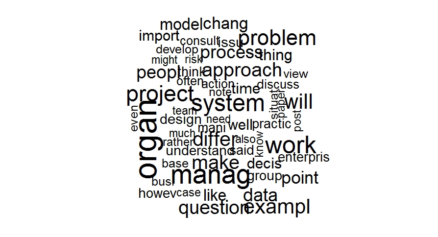
Fig 2: Wordcloud (freq>70)
Here we first load the wordcloud package which is not loaded by default. Setting a seed number ensures that you get the same look each time (try running it without setting a seed). The arguments of the wordcloud() function are straightforward enough. Note that one can specify the maximum number of words to be included instead of the minimum frequency (as I have done above). See the word cloud documentation for more.
This word cloud also makes it clear that stop word removal has not done its job well, there are a number of words it has missed (also and however, for example). These can be removed by augmenting the built-in stop word list with a custom one. This is left as an exercise for the reader :-).
Finally, one can make the wordcloud more visually appealing by adding colour as follows:
wordcloud(names(freqr),freqr,min.freq=70,colors=brewer.pal(6,”Dark2″))
The result is shown Figure 3.

Fig 3: Wordcloud (freq > 70)
You may need to load the RColorBrewer package to get this to work. Check out the brewer documentation to experiment with more colouring options.
Wrapping up
This brings me to the end of this rather long (but I hope, comprehensible) introduction to text mining R. It should be clear that despite the length of the article, I’ve covered only the most rudimentary basics. Nevertheless, I hope I’ve succeeded in conveying a sense of the possibilities in the vast and rapidly-expanding discipline of text analytics.
Note added on July 22nd, 2015:
If you liked this piece, you may want to check out the sequel – a gentle introduction to cluster analysis using R.
Note added on September 29th 2015:
…and my introductory piece on topic modeling.
Note added on December 3rd 2015:
…and my article on visualizing relationships between documents.
Beyond entities and relationships – towards an emergent approach to data modelling
Introduction – some truths about data modelling
It has been said that data is the lifeblood of business. The aptness of this metaphor became apparent to when I was engaged in a data mapping project some years ago. The objective of that effort was to document all the data flows within the organization. The final map showed very clearly that the volume of data on the move was good indicator of the activity of the function: the greater the volume, the more active the function. This is akin to the case of the human body wherein organs that expend the more energy tend to have a richer network of blood vessels.
Although the above analogy is far from perfect, it serves to highlight the simple fact that most business activities involve the movement and /or processing of data. Indeed, the key function of information systems that support business activities is to operate on and transfer data. It therefore matters a lot as to how data is represented and stored. This is the main concern of the discipline of data modelling.
The mainstream approach to data modelling assumes that real world objects and relationships can be accurately represented by models. As an example, a data model representing a sales process might consist of entities such as customers and products and their relationships, such as sales (customer X purchases product Y). It is tacitly assumed that objective, bias-free models of entities and relationships of interest can be built by asking the right questions and using appropriate information collection techniques.
However, things are not quite so straightforward: as professional data modellers know, real-world data models are invariably tainted by compromises between rigour and reality. This is inevitable because the process of building a data model involves at least two different sets of stakeholders whose interests are often at odds – namely, business users and data modelling professionals. The former are less interested in the purity of model than the business process that it is intended to support; the interests of the latter, however, are often the opposite.
This reveals a truth about data modelling that is not fully appreciated by practitioners: that it is a process of negotiation rather than a search for a true representation of business reality. In other words, it is a socio-technical problem that has wicked elements. As such then, data modelling ought to be based on the principles of emergent design. In this post I explore this idea drawing on a brilliant paper by Heinz Klein and Kalle Lyytinen entitled, Towards a New Understanding of Data Modelling as well as my own thoughts on the subject.
Background
Klein and Lyytinen begin their paper by asking four questions that are aimed at uncovering the tacit assumptions underlying the different approaches to data modelling. The questions are:
- What is being modelled? This question delves into the nature of the “universe” that a data model is intended to represent.
- How well is the result represented? This question asks if the language, notations and symbols used to represent the results are fit for purpose – i.e. whether the language and constructs used are capable of modelling the domain.
- Is the result valid? This asks the question as to whether the model is a correct representation of the domain that is being modelled.
- What is the social context in which the discipline operates? This question is aimed at eliciting the views of different stakeholders regarding the model: how they will use it, whether their interests are taken into account and whether they benefit or lose from it.
It should be noted that these questions are general in that they can be used to enquire into any discipline. In the next section we use these questions to uncover the tacit assumptions underlying the mainstream view of data modelling. Following that, we propose an alternate set of assumptions that address a major gap in the mainstream view.
Deconstructing the mainstream view
What is being modelled?
As Klein and Lyytinen put it, the mainstream approach to data modelling assumes that the world is given and made up of concrete objects which have natural properties and are associated with [related to] other objects. This assumption is rooted in a belief that it is possible to build an objectively true picture of the world around us. This is pretty much how truth is perceived in data modelling: data/information is true or valid if it describes something – a customer, an order or whatever – as it actually is.
In philosophy, such a belief is formalized in the correspondence theory of truth, a term that refers to a family of theories that trace their origins back to antiquity. According to Wikipedia:
Correspondence theories claim that true beliefs and true statements correspond to the actual state of affairs. This type of theory attempts to posit a relationship between thoughts or statements on one hand, and things or facts on the other. It is a traditional model which goes back at least to some of the classical Greek philosophers such as Socrates, Plato, and Aristotle. This class of theories holds that the truth or the falsity of a representation is determined solely by how it relates to a reality; that is, by whether it accurately describes that reality.
In short: the mainstream view of data modelling is based on the belief that the things being modelled have an objective existence.
How well is the result represented?
If data models are to represent reality (as it actually is), then one also needs an appropriate means to express that reality in its entirety. In other words, data models must be complete and consistent in that they represent the entire domain and do not contain any contradictory elements. Although this level of completeness and logical rigour is impossible in practice, much research effort is expended in finding evermore complete and logical consistent notations.
Practitioners have little patience with cumbersome notations invented by theorists, so it is no surprise that the most popular modelling notation is the simplest one: the entity-relationship (ER) approach which was first proposed by Peter Chen. The ER approach assumes that the world can be represented by entities (such as customer) with attributes (such as name), and that entities can be related to each other (for example, a customer might be located at an address – here “is located at” is a relationship between the customer and address entities). Most commercial data modelling tools support this notation (and its extensions) in one form or another.
To summarise: despite the fact that the most widely used modelling notation is not based on rigorous theory, practitioners generally assume that the ER notation is an appropriate vehicle to represent what is going on in the domain of interest.
Is the result valid?
As argued above, the mainstream approach to data modelling assumes that the world of interest has an objective existence and can be represented by a simple notation that depicts entities of interest and the relationships between them. This leads to the question of the validity of the models thus built. To answer this we have to understand how data models are constructed.
The process of model-building involves observation, information gathering and analysis – that is, it is akin to the approach used in scientific enquiry. A great deal of attention is paid to model verification, and this is usually done via interaction with subject matter experts, users and business analysts. To be sure, the initial model is generally incomplete, but it is assumed that it can be iteratively refined to incorporate newly surfaced facts and fix errors. The underlying belief is that such a process gets ever-closer to the truth.
In short: it is assumed that it an ER model built using a systematic and iterative process of enquiry will result in a model that is a valid representation of the domain of interest.
What is the social context in which the discipline operates?
From the above, one might get the impression that data modelling involves a lot of user interaction. Although this is generally true, it is important to note that the users’ roles are restricted to providing information to data modellers. The modellers then interpret the information provided by users and cast into a model.
This brings up an important socio-political implication of the mainstream approach: data models generally support business applications that are aimed at maintaining and enhancing managerial control through automation and / or improved oversight. Underlying this is the belief that a properly constructed data model (i.e. one that accurately represents reality) can enhance business efficiency and effectiveness within the domain represented by the model.
In brief: data models are built to further the interests of specific stakeholder groups within an organization.
Summarising the mainstream view
The detailed responses to the questions above reveal that the discipline of data modelling is based on the following assumptions:
- The domain of interest has an objective existence.
- The domain can be represented using a (more or less) logical language.
- The language can represent the domain of interest accurately.
- The resulting model is based largely on a philosophy of managerial control, and can be used to drive organizational efficiency and effectiveness.
Many (most?) professional data management professionals will see these assumptions as being uncontroversial. However, as we shall see next, things are not quite so simple…
Motivating an alternate view of data modelling
In an earlier section I mentioned the correspondence theory of truth which tells us that true statements are those that correspond to the actual state of affairs in the real world. A problem with correspondence theories is that they assume that: a) there is an objective reality, and b) that it is perceived in the same way by everyone. This assumption is problematic, especially for issues that have a social dimension. Such issues are perceived differently by different stakeholders, each of who will seek data that supports their point of view. The problem is that there is no way to determine which data is “objectively right.” More to the point, in such situations the very notion of “objective rightness” can be legitimately questioned.
Another issue with correspondence theories is that a piece of data can at best be an abstraction of a real-world object or event. This is a serious problem with correspondence theories in the context of business intelligence. For example, when a sales rep records a customer call, he or she notes down only what is required by the CRM system. Other data that may well be more important is not captured or is relegated to a “Notes” or “Comments” field that is rarely if ever searched or accessed.
Another perspective on truth is offered by the so called consensus theory which asserts that true statement are those that are agreed to by the relevant group of people. This is often the way “truth” is established in organisations. For example, managers may choose to calculate KPIs using certain pieces of data that are deemed to be true. The problem with this is that consensus can be achieved by means that are not necessarily democratic .For example, a KPI definition chosen by a manager may be contested by an employee. Nevertheless, the employee has to accept it because organisations are not democracies. A more significant issue is that the notion of “relevant group” is problematic because there is no clear criterion by which to define relevance. Quite naturally this leads to conflict and ill-will.
This conclusion leads one to formulate alternative answers to four questions posed above, thus paving the way to a new approach to data modelling.
An alternate view of data management
What is being modelled?
The discussion of the previous section suggests that data models cannot represent an objective reality because there is never any guarantee that all interested parties will agree on what that reality is. Indeed, insofar as data models are concerned, it is more useful to view reality as being socially constructed – i.e. collectively built by all those who have a stake in it.
How is reality socially constructed? Basically it is through a process of communication in which individuals discuss their own viewpoints and agree on how differences (if any) can be reconciled. The authors note that:
…the design of an information system is not a question of fitness for an organizational reality that can be modelled beforehand, but a question of fitness for use in the construction of a [collective] organizational reality…
This is more in line with the consensus theory of truth than the correspondence theory.
In brief: the reality that data models are required to represent is socially constructed.
How well is the result represented?
Given the above, it is clear that any data model ought to be subjected to validation by all stakeholders so that they can check that it actually does represent their viewpoint. This can be difficult to achieve because most stakeholders do not have the time or inclination to validate data models in detail.
In view of the above, it is clear that the ER notation and others of its ilk can represent a truth rather than the truth – that is, they are capable of representing the world according to a particular set of stakeholders (managers or users, for example). Indeed, a data model (in whatever notation) can be thought of one possible representation of a domain. The point is, there are as many representations possible as there are stakeholder groups and in mainstream data modelling, and one of these representations “wins” while the others are completely ignored. Indeed, the alternate views generally remain undocumented so they are invariably forgotten. This suggests that a key step in data modelling would be to capture all possible viewpoints on the domain of interest in a way that makes a sensible comparison possible. Apart from helping the group reach a consensus, such documentation is invaluable to explain to future users and designers why the data model is the way it is. Regular readers of this blog will no doubt see that the IBIS notation and dialogue mapping could be hugely helpful in this process. It would take me too far afield to explore this point here, but I will do so in a future post.
In brief: notations used by mainstream data modellers cannot capture multiple worldviews in a systematic and useful way. These conventional data modelling languages need to be augmented by notations that are capable of incorporating diverse viewpoints.
Is the result valid?
The above discussion begs a question, though: what if two stakeholders disagree on a particular point?
One answer to this lies in Juergen Habermas’ theory of communicative rationaility that I have discussed in detail in this post. I’ll explain the basic idea via the following excerpt from that post:
When we participate in discussions we want our views to be taken seriously. Consequently, we present our views through statements that we hope others will see as being rational – i.e. based on sound premises and logical thought. One presumes that when someone makes claim, he or she is willing to present arguments that will convince others of the reasonableness of the claim. Others will judge the claim based the validity of the statements claimant makes. When the validity claims are contested, debate ensues with the aim of getting to some kind of agreement.
The philosophy underlying such a process of discourse (which is simply another word for “debate” or “dialogue”) is described in the theory of communicative rationality proposed by the German philosopher Jurgen Habermas. The basic premise of communicative rationality is that rationality (or reason) is tied to social interactions and dialogue. In other words, the exercise of reason can occur only through dialogue. Such communication, or mutual deliberation, ought to result in a general agreement about the issues under discussion. Only once such agreement is achieved can there be a consensus on actions that need to be taken. Habermas refers to the latter as communicative action, i.e. action resulting from collective deliberation…
In brief: validity is not an objective matter but a subjective – or rather an intersubjective one that is, validity has to be agreed between all parties affected by the claim.
What is the social context in which the discipline operates?
From the above it should be clear that the alternate view of data management is radically different from the mainstream approach. The difference is particularly apparent when one looks at the way in which the alternate approach views different stakeholder groups. Recall that in the mainstream view, managerial perspectives take precedence over all others because the overriding aim of data modelling (as indeed most enterprise IT activities) is control. Yes, I am aware that it is supposed to be about enablement, but the question is enablement for whom? In most cases, the answer is that it enables managers to control. In contrast, from the above we see that the reality depicted in a data (or any other) model is socially constructed – that is, it is based on a consensus arising from debates on the spectrum of views that people hold. Moreover, no claim has precedence over others on virtue of authority. Different interpretations of the world have to be fused together in order to build a consensually accepted world.
The social aspect is further muddied by conflicts between managers on matters of data ownership, interpretation and access. Typically, however, such matters lie outside the purview of data modellers
In brief: the social context in which the discipline operates is that there are a wide variety of stakeholder groups, each of which may hold different views. These must be debated and reconciled.
Summarising the alternate view
The detailed responses to the questions above reveal that the alternate view of data modelling is based on the following assumptions:
- The domain of interest is socially constructed.
- The standard representations of data models are inadequate because they cannot represent multiple viewpoints. They can (and should) be supplemented by notations that can document multiple viewpoints.
- A valid data model is constructed through an iterative synthesis of multiple viewpoints.
- The resulting model is based on a shared understanding of the socially constructed domain.
Clearly these assumptions are diametrically opposed to those in the mainstream. Let’s briefly discuss their implications for the profession
Discussion
The most important implication of the alternate view is that a data model is but one interpretation of reality. As such, there are many possible interpretations of reality and the “correctness” of any particular model hinges not on some objective truth but on an agreed, best-for-group interpretation. A consequence of the above is that well-constructed data models “fuse” or “bring together” at least two different interpretations – those of users and modellers. Typically there are many different groups of users, each with their own interpretation. This being the case, it is clear that the onus lies on modellers to reconcile any differences between these groups as they are the ones responsible for creating models.
A further implication of the above is that it is impossible to build a consistent enterprise-wide data model. That said, it is possible to have a high-level strategic data model that consists, say, of entities but lacks detailed attribute-level information. Such a model can be useful because it provides a starting point for a dialogue between user groups and also serves to remind modellers of the entities they may need to consider when building a detailed data model.
The mainstream view asserts that data is gathered to establish the truth. The alternate view, however, makes us aware that data models are built in such a way as to support particular agendas. Moreover, since the people who use the data are not those who collect or record it, a gap between assumed and actual meaning is inevitable. Once again this emphasises that fact that the meaning of a particular piece of data is very much in the eye of the beholder.
In closing
The mainstream approach to data modelling reflects the general belief that the methods of natural sciences can be successfully applied in the area of systems development. Although this is a good assumption for theoretical computer science, which deals with constructs such as data structures and algorithms, it is highly questionable when it comes to systems development in large organisations. In the latter case social factors dominate, and these tend to escape any logical system. This simple fact remains under-appreciated by the data modelling community and, for that matter, much of the universe of corporate IT.
The alternate view described in this post draws attention to the social and political aspects of data modelling. Although IT vendors and executives tend to give these issues short shrift, the chronically high failure rate of data-centric initiatives (such as those aimed at building enterprise data warehouses) warns us to pause and think. If there is anything at all to be learnt from these failures, it is that data modelling is not a science that deals with facts and models, but an art that has more to do with negotiation and law-making.


