Archive for the ‘Data Science’ Category
A gentle introduction to random forests using R
Introduction
In a previous post, I described how decision tree algorithms work and demonstrated their use via the rpart library in R. Decision trees work by splitting a dataset recursively. That is, subsets arising from a split are further split until a predetermined termination criterion is reached. At each step, a split is made based on the independent variable that results in the largest possible reduction in heterogeneity of the dependent variable.
(Note: readers unfamiliar with decision trees may want to read that post before proceeding)
The main drawback of decision trees is that they are prone to overfitting. The reason for this is that trees, if grown deep, are able to fit all kinds of variations in the data, including noise. Although it is possible to address this partially by pruning, the result often remains less than satisfactory. This is because the algorithm makes a locally optimal choice at each split without any regard to whether the choice made is the best one overall. A poor split made in the initial stages can thus doom the model, a problem that cannot be fixed by post-hoc pruning.
In this post I describe random forests, a tree-based algorithm that addresses the above shortcoming of decision trees. I’ll first describe the intuition behind the algorithm via an analogy and then do a demo using the R randomForest library.
Motivating random forests
One of the reasons for the popularity of decision trees is that they reflect the way humans make decisions: by weighing up options at each stage and choosing the best one available. The analogy is particularly useful because it also suggests how decision trees can be improved.
One of the lifelines in the game show, Who Wants to be A Millionaire, is “Ask The Audience” wherein a contestant can ask the audience to vote on the answer to a question. The rationale here is that the majority response from a large number of independent decision makers is more likely to yield a correct answer than one from a randomly chosen person. There are two factors at play here:
- People have different experiences and will therefore draw upon different “data” to answer the question.
- People have different knowledge bases and preferences and will therefore draw upon different “variables” to make their choices at each stage in their decision process.
Taking a cue from the above, it seems reasonable to build many decision trees using:
- Different sets of training data.
- Randomly selected subsets of variables at each split of every decision tree.
Predictions can then made by taking the majority vote over all trees (for classification problems) or averaging results over all trees (for regression problems). This is essentially how the random forest algorithm works.
The net effect of the two strategies is to reduce overfitting by a) averaging over trees created from different samples of the dataset and b) decreasing the likelihood of a small set of strong predictors dominating the splits. The price paid is reduced interpretability as well as increased computational complexity. But then, there is no such thing as a free lunch.
The mechanics of the algorithm
Although we will not delve into the mathematical details of the algorithm, it is important to understand how two points made above are implemented in the algorithm.
Bootstrap aggregating… and a (rather cool) error estimate
A key feature of the algorithm is the use of multiple datasets for training individual decision trees. This is done via a neat statistical trick called bootstrap aggregating (also called bagging).
Here’s how bagging works:
Assume you have a dataset of size N. From this you create a sample (i.e. a subset) of size n (n less than or equal to N) by choosing n data points randomly with replacement. “Randomly” means every point in the dataset is equally likely to be chosen and “with replacement” means that a specific data point can appear more than once in the subset. Do this M times to create M equally-sized samples of size n each. It can be shown that this procedure, which statisticians call bootstrapping, is legit when samples are created from large datasets – that is, when N is large.
Because a bagged sample is created by selection with replacement, there will generally be some points that are not selected. In fact, it can be shown that, on the average, each sample will use about two-thirds of the available data points. This gives us a clever way to estimate the error as part of the process of model building.
Here’s how:
For every data point, obtain predictions for trees in which the point was out of bag. From the result mentioned above, this will yield approximately M/3 predictions per data point (because a third of the data points are out of bag). Take the majority vote of these M/3 predictions as the predicted value for the data point. One can do this for the entire dataset. From these out of bag predictions for the whole dataset, we can estimate the overall error by computing a classification error (Count of correct predictions divided by N) for classification problems or the root mean squared error for regression problems. This means there is no need to have a separate test data set, which is kind of cool. However, if you have enough data, it is worth holding out some data for use as an independent test set. This is what we’ll do in the demo later.
Using subsets of predictor variables
Although bagging reduces overfitting somewhat, it does not address the issue completely. The reason is that in most datasets a small number of predictors tend to dominate the others. These predictors tend to be selected in early splits and thus influence the shapes and sizes of a significant fraction of trees in the forest. That is, strong predictors enhance correlations between trees which tends to come in the way of variance reduction.
A simple way to get around this problem is to use a random subset of variables at each split. This avoids over-representation of dominant variables and thus creates a more diverse forest. This is precisely what the random forest algorithm does.
Random forests in R
In what follows, I use the famous Glass dataset from the mlbench library. The dataset has 214 data points of six types of glass with varying metal oxide content and refractive indexes. I’ll first build a decision tree model based on the data using the rpart library (recursive partitioning) that I covered in an earlier article and then use then show how one can build a random forest model using the randomForest library. The rationale behind this is to compare the two models – single decision tree vs random forest. In the interests of space, I won’t explain details of the rpart here as I’ve covered it at length in the previous article. However, for completeness, I’ll list the demo code for it before getting into random forests.
Decision trees using rpart
Here’s the code listing for building a decision tree using rpart on the Glass dataset (please see my previous article for a full explanation of each step). Note that I have not used pruning as there is little benefit to be gained from it (Exercise for the reader: try this for yourself!).
Now, we know that decision tree algorithms tend to display high variance so the hit rate from any one tree is likely to be misleading. To address this we’ll generate a bunch of trees using different training sets (via random sampling) and calculate an average hit rate and spread (or standard deviation).
The decision tree algorithm gets it right about 69% of the time with a variation of about 5%. The variation isn’t too bad here, but the accuracy has hardly improved at all (Exercise for the reader: why?). Let’s see if we can do better using random forests.
Random forests
As discussed earlier, a random forest algorithm works by averaging over multiple trees using bootstrapped samples. Also, it reduces the correlation between trees by splitting on a random subset of predictors at each node in tree construction. The key parameters for randomForest algorithm are the number of trees (ntree) and the number of variables to be considered for splitting (mtry). The algorithm sets a default of 500 for ntree and sets mtry to the square root of the the number of predictors for classification problems or one-third the total number of predictors for regression. These defaults can be overridden by explicitly providing values for these variables.
The preliminary stuff – the creation of training and test datasets etc. – is much the same as for decision trees but I’ll list the code for completeness.
randomForest(formula = Type ~ ., data = trainGlass, importance = TRUE, xtest = testGlass[, -typeColNum], ntree = 1001)
| 1 | 2 | 3 | 5 | 6 | 7 | class.error | |
| 1 | 40 | 7 | 2 | 0 | 0 | 0 | 0.1836735 |
| 2 | 8 | 49 | 1 | 2 | 2 | 1 | 0.2222222 |
| 3 | 6 | 3 | 6 | 0 | 0 | 0 | 0.6000000 |
| 5 | 0 | 1 | 0 | 11 | 0 | 1 | 0.1538462 |
| 6 | 1 | 2 | 0 | 1 | 6 | 0 | 0.5000000 |
| 7 | 1 | 2 | 0 | 1 | 0 | 21 | 0.1600000 |
The first thing to note is the out of bag error estimate is ~ 24%. Equivalently the hit rate is 76%, which is better than the 69% for decision trees. Secondly, you’ll note that the algorithm does a terrible job identifying type 3 and 6 glasses correctly. This could possibly be improved by a technique called boosting, which works by iteratively improving poor predictions made in earlier stages. I plan to look at boosting in a future post, but if you’re curious, check out the gbm package in R.
Finally, for completeness, let’s see how the test set does:
| 1 | 2 | 3 | 5 | 6 | 7 | |
| 1 | 19 | 2 | 0 | 0 | 0 | 0 |
| 2 | 1 | 9 | 1 | 0 | 0 | 0 |
| 3 | 1 | 1 | 1 | 0 | 0 | 0 |
| 5 | 0 | 1 | 0 | 0 | 0 | 0 |
| 6 | 0 | 0 | 0 | 0 | 3 | 0 |
| 7 | 0 | 0 | 0 | 0 | 0 | 4 |
The test accuracy is better than the out of bag accuracy and there are some differences in the class errors as well. However, overall the two compare quite well and are significantly better than the results of the decision tree algorithm.
Variable importance
Random forest algorithms also give measures of variable importance. Computation of these is enabled by setting importance, a boolean parameter, to TRUE. The algorithm computes two measures of variable importance: mean decrease in Gini and mean decrease in accuracy. Brief explanations of these follow.
Mean decrease in Gini
When determining splits in individual trees, the algorithm looks for the largest class (in terms of population) and attempts to isolate it first. If this is not possible, it tries to do the best it can, always focusing on isolating the largest remaining class in every split.This is called the Gini splitting rule (see this article for a good explanation of the rule).
The “goodness of split” is measured by the Gini Impurity, 

where 


Mean decrease in accuracy
The mean decrease in accuracy is calculated using the out of bag data points for each tree. The procedure goes as follows: when a particular tree is grown, the out of bag points are passed down the tree and the prediction accuracy (based on all out of bag points) recorded . The predictors are then randomly permuted and the out of bag prediction accuracy recalculated. The decrease in accuracy for a given predictor is the difference between the accuracy of the original (unpermuted) tree and the those obtained from the permuted trees in which the predictor was excluded. As in the previous case, the decrease in accuracy for each predictor can be computed and tracked as the algorithm progresses. These can then be averaged by predictor to yield a mean decrease in accuracy.
Variable importance plot
From the above, it would seem that the mean decrease in accuracy is a more global measure as it uses fully constructed trees in contrast to the Gini measure which is based on individual splits. In practice, however, there could be other reasons for choosing one over the other…but that is neither here nor there, if you set importance to TRUE, you’ll get both. The numerical measures of importance are returned in the randomForest object (Glass.rf in our case), but I won’t list them here. Instead, I’ll just print out the variable importance plots for the two measures as these give a good visual overview of the relative importance of variables. The code is a simple one-liner:
The plot is shown in Figure 1 below.

Figure 1: Variable importance plots
In this case the two measures are pretty consistent so it doesn’t really matter which one you choose.
Wrapping up
Random forests are an example of a general class of techniques called ensemble methods. These techniques are based on the principle that averaging over a large number of not-so-good models yields a more reliable prediction than a single model. This is true only if models in the group are independent of each other, which is precisely what bootstrap aggregation and predictor subsetting are intended to achieve.
Although considerably more complex than decision trees, the logic behind random forests is not hard to understand. Indeed, the intuitiveness of the algorithm together with its ease of use and accuracy have made it very popular in the machine learning community.
The story before the story – a data science fable
It is well-known that data-driven stories are a great way to convey results of data science initiatives. What is perhaps not as well-known is that data science projects often have to begin with stories too. Without this “story before the story” there will be no project, no results and no data-driven stories to tell….
For those who prefer to read, here’s a transcript of the video in full:
In the beginning there is no data, let alone results…but there are ideas. So, long before we tell stories about data or results, we have to tell stories about our ideas. The aim of these stories is to get people to care about our ideas as much as we do and, more important, invest in them. Without their interest or investment there will be no results and no further stories to tell.
So one of the first things one has to do is craft a story about the idea…or the story before the story.
Once upon a time there was a CRM system. The system captured every customer interaction that occurred, whether it was by phone, email or face to face conversation. Many quantitative details of interactions were recorded, time, duration, type. And if the interaction led to a sale, the details of the sale were recorded too.
Almost as an aside, the system also gave sales people the opportunity to record their qualitative impressions as free text notes. As you might imagine, this information, though potentially valuable, was never analysed. Sure managers looked at notes in isolation from time to time when referring.to specific customer interactions, but there was no systematic analysis of the corpus as a whole. Nobody had thought it worthwhile to do this, possibly because it is difficult if not quite impossible to analyse unstructured information in the world of relational databases and SQL.
One day, an analyst was browsing data randomly in the system, as good analysts sometimes do. He came across a note that to him seemed like the epitome of a good note…it described what the interaction was about, the customer’s reactions and potential next steps all in a logical fashion.
This gave him an idea. Wouldn’t it be cool, he thought, if we could measure the quality of notes? Not only would this tell us something about the customer and the interaction, it may tell us something about the sales person as well.
The analyst was mega excited…but he realised he’d need help. He was an IT guy and as we all know, business folks in big corporations stopped listening to their IT guys long ago. So our IT guy had his work cut out for him.
After much cogitation, he decided to enlist the help of his friend, a strategic business analyst in the marketing department. This lady, who worked in marketing had the trust of the head of marketing. If she liked the idea, she might be able to help sell it to the head of marketing.
As it turned out, the business analyst loved the idea…more important, since she knew what the sales people do on a day to day basis, she could give the IT guy more ideas on how he could build quantitative measures of the quality of notes. For example, she suggested looking for emotion-laden words or mentions of competitor’s products and so on. The IT guy now had some concrete things to work on. The initial results gave them even more ideas, and soon they had more than enough to make a convincing pitch to the head of marketing.
It would take us too far afield to discuss details of the pitch, but what we will say is this: they avoided technical details, instead focusing on the strategic and innovative aspects of the work.
The marketing head liked the idea…what was there not to like? He agreed to support the effort, and the idea became a project….
…and yes, within months the project resulted in new insights into customer behaviour. But that is another story.
A gentle introduction to decision trees using R
Introduction
Most techniques of predictive analytics have their origins in probability or statistical theory (see my post on Naïve Bayes, for example). In this post I’ll look at one that has more a commonplace origin: the way in which humans make decisions. When making decisions, we typically identify the options available and then evaluate them based on criteria that are important to us. The intuitive appeal of such a procedure is in no small measure due to the fact that it can be easily explained through a visual. Consider the following graphic, for example:

Figure 1: Example of a simple decision tree (Courtesy: Duncan Hull)
(Original image: https://www.flickr.com/photos/dullhunk/7214525854, Credit: Duncan Hull)
The tree structure depicted here provides a neat, easy-to-follow description of the issue under consideration and its resolution. The decision procedure is based on asking a series of questions, each of which serve to further reduce the domain of possibilities. The predictive technique I discuss in this post,classification and regression trees (CART), works in much the same fashion. It was invented by Leo Breiman and his colleagues in the 1970s.
In what follows, I will use the open source software, R. If you are new to R, you may want to follow this link for more on the basics of setting up and installing it. Note that the R implementation of the CART algorithm is called RPART (Recursive Partitioning And Regression Trees). This is essentially because Breiman and Co. trademarked the term CART. As some others have pointed out, it is somewhat ironical that the algorithm is now commonly referred to as RPART rather than by the term coined by its inventors.
A bit about the algorithm
The rpart algorithm works by splitting the dataset recursively, which means that the subsets that arise from a split are further split until a predetermined termination criterion is reached. At each step, the split is made based on the independent variable that results in the largest possible reduction in heterogeneity of the dependent (predicted) variable.
Splitting rules can be constructed in many different ways, all of which are based on the notion of impurity- a measure of the degree of heterogeneity of the leaf nodes. Put another way, a leaf node that contains a single class is homogeneous and has impurity=0. There are three popular impurity quantification methods: Entropy (aka information gain), Gini Index and Classification Error. Check out this article for a simple explanation of the three methods.
The rpart algorithm offers the entropy and Gini index methods as choices. There is a fair amount of fact and opinion on the Web about which method is better. Here are some of the better articles I’ve come across:
https://www.garysieling.com/blog/sklearn-gini-vs-entropy-criteria
http://www.salford-systems.com/resources/whitepapers/114-do-splitting-rules-really-matter
The answer as to which method is the best is: it depends. Given this, it may be prudent to try out a couple of methods and pick the one that works best for your problem.
Regardless of the method chosen, the splitting rules partition the decision space (a fancy word for the entire dataset) into rectangular regions each of which correspond to a split. Consider the following simple example with two predictors x1 and x2. The first split is at x1=1 (which splits the decision space into two regions x11), the second at x2=2, which splits the (x1>1) region into 2 sub-regions, and finally x1=1.5 which splits the (x1>1,x2>2) sub-region further.
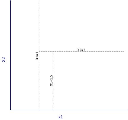
Figure 2: Example of partitioning
It is important to note that the algorithm works by making the best possible choice at each particular stage, without any consideration of whether those choices remain optimal in future stages. That is, the algorithm makes a locally optimal decision at each stage. It is thus quite possible that such a choice at one stage turns out to be sub-optimal in the overall scheme of things. In other words, the algorithm does not find a globally optimal tree.
Another important point relates to well-known bias-variance tradeoff in machine learning, which in simple terms is a tradeoff between the degree to which a model fits the training data and its predictive accuracy. This refers to the general rule that beyond a point, it is counterproductive to improve the fit of a model to the training data as this increases the likelihood of overfitting. It is easy to see that deep trees are more likely to overfit the data than shallow ones. One obvious way to control such overfitting is to construct shallower trees by stopping the algorithm at an appropriate point based on whether a split significantly improves the fit. Another is to grow a tree unrestricted and then prune it back using an appropriate criterion. The rpart algorithm takes the latter approach.
Here is how it works in brief:
Essentially one minimises the cost, 


First, we note that when 

An implication of their tendency to overfit data is that decision trees tend to be sensitive to relatively minor changes in the training datasets. Indeed, small differences can lead to radically different looking trees. Pruning addresses this to an extent, but does not resolve it completely. A better resolution is offered by the so-called ensemble methods that average over many differently constructed trees. I’ll discuss one such method at length in a future post.
Finally, I should also mention that decision trees can be used for both classification and regression problems (i.e. those in which the predicted variable is discrete and continuous respectively). I’ll demonstrate both types of problems in the next two sections.
Classification trees using rpart
To demonstrate classification trees, we’ll use the Ionosphere dataset available in the mlbench package in R. I have chosen this dataset because it nicely illustrates the points I wish to make in this post. In general, you will almost always find that algorithms that work fine on classroom datasets do not work so well in the real world…but of course, you know that already!
We begin by setting the working directory, loading the required packages (rpart and mlbench) and then loading the Ionosphere dataset.
Next we separate the data into training and test sets. We’ll use the former to build the model and the latter to test it. To do this, I use a simple scheme wherein I randomly select 80% of the data for the training set and assign the remainder to the test data set. This is easily done in a single R statement that invokes the uniform distribution (runif) and the vectorised function, ifelse. Before invoking runif, I set a seed integer to my favourite integer in order to ensure reproducibility of results.
In the above, I have also removed the training flag from the training and test datasets.
Next we invoke rpart. I strongly recommend you take some time to go through the documentation and understand the parameters and their defaults values. Note that we need to remove the predicted variable from the dataset before passing the latter on to the algorithm, which is why we need to find the column index of the predicted variable (first line below). Also note that we set the method parameter to “class“, which simply tells the algorithm that the predicted variable is discrete. Finally, rpart uses Gini rule for splitting by default, and we’ll stick with this option.
The resulting plot is shown in Figure 3 below. It is quite self-explanatory so I won’t dwell on it here.
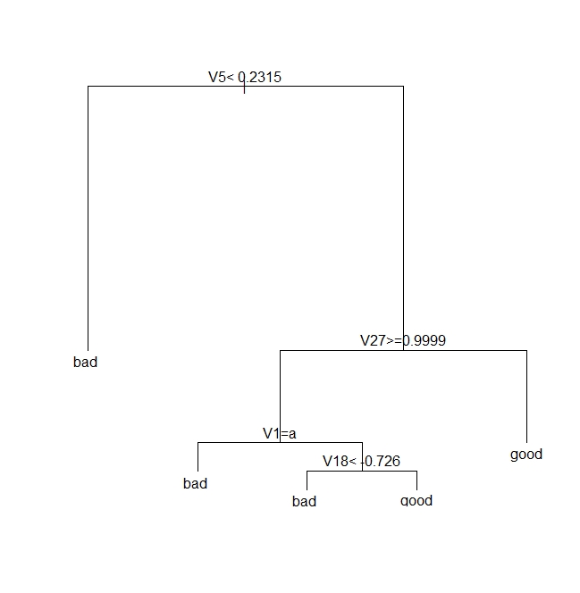
Figure 3: A classification tree for Ionosphere dataset
Next we see how good the model is by seeing how it fares against the test data.
| pred true | bad | good |
| bad | 17 | 2 |
| good | 9 | 43 |
Note that we need to verify the above results by doing multiple runs, each using different training and test sets. I will do this later, after discussing pruning.
Next, we prune the tree using the cost complexity criterion. Basically, the intent is to see if a shallower subtree can give us comparable results. If so, we’d be better of choosing the shallower tree because it reduces the likelihood of overfitting.
As described earlier, we choose the appropriate pruning parameter (aka cost-complexity parameter)
| CP | nsplit | rel error | xerror | xstd | |
| 1 | 0.57 | 0 | 1.00 | 1.00 | 0.080178 |
| 2 | 0.20 | 1 | 0.43 | 0.46 | 0.062002 |
| 3 | 0.02 | 2 | 0.23 | 0.26 | 0.048565 |
| 4 | 0.01 | 4 | 0.19 | 0.35 |
It is clear from the above, that the lowest cross-validation error (xerror in the table) occurs for 
Next, we prune the tree based on this value of CP:
Note that rpart will use a default CP value of 0.01 if you don’t specify one in prune.
The pruned tree is shown in Figure 4 below.

Figure 4: A pruned classification tree for Ionosphere dataset
Let’s see how this tree stacks up against the fully grown one shown in Fig 3.
This seems like an improvement over the unpruned tree, but one swallow does not a summer make. We need to check that this holds up for different training and test sets. This is easily done by creating multiple random partitions of the dataset and checking the efficacy of pruning for each. To do this efficiently, I’ll create a function that takes the training fraction, number of runs (partitions) and the name of the dataset as inputs and outputs the proportion of correct predictions for each run. It also optionally prunes the tree. Here’s the code:
Note that in the above, I have set the default value of the prune_tree to FALSE, so the function will execute the first branch of the if statement unless the default is overridden.
OK, so let’s do 50 runs with and without pruning, and check the mean and variance of the results for both sets of runs.
So we see that there is an improvement of about 3% with pruning. Also, if you were to plot the trees as we did earlier, you would see that this improvement is achieved with shallower trees. Again, I point out that this is not always the case. In fact, it often happens that pruning results in worse predictions, albeit with better reliability – a classic illustration of the bias-variance tradeoff.
Regression trees using rpart
In the previous section we saw how one can build decision trees for situations in which the predicted variable is discrete. Let’s now look at the case in which the predicted variable is continuous. We’ll use the Boston Housing dataset from the mlbench package. Much of the discussion of the earlier section applies here, so I’ll just display the code, explaining only the differences.
Next we invoke rpart, noting that the predicted variable is medv (median value of owner-occupied homes in $1000 units) and that we need to set the method parameter to “anova“. The latter tells rpart that the predicted variable is continuous (i.e that this is a regression problem).
The plot of the tree is shown in Figure 5 below.
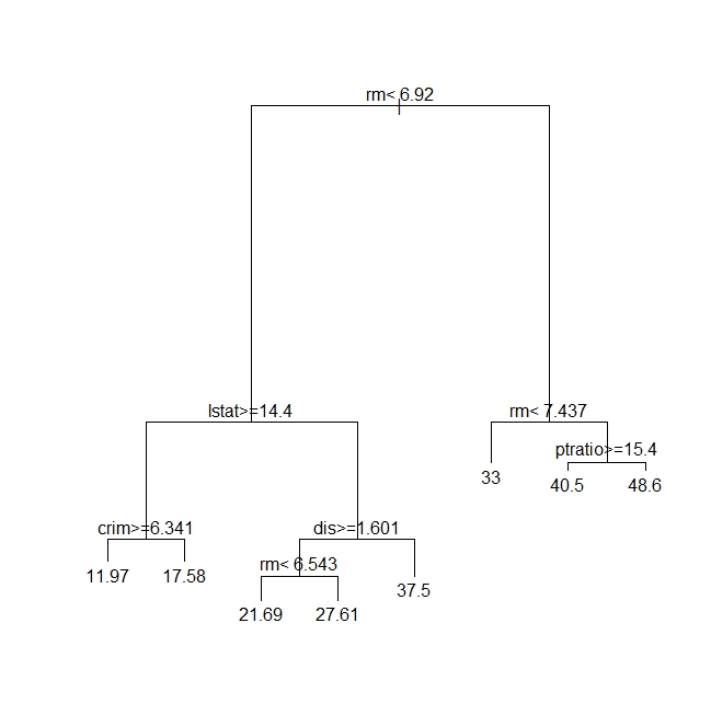
Figure 5: A regression tree for Boston Housing dataset
Next, we need to see how good the predictions are. Since the dependent variable is continuous, we cannot compare the predictions directly against the test set. Instead, we calculate the root mean square (RMS) error. To do this, we request rpart to output the predictions as a vector – one prediction per record in the test dataset. The RMS error can then easily be calculated by comparing this vector with the medv column in the test dataset.
Here is the relevant code:
Again, we need to do multiple runs to check on the reliability of the predictions. However, you already know how to do that so I will leave it to you.
Moving on, we prune the tree using the cost complexity criterion as before. The code is exactly the same as in the classification problem.
The tree is unchanged so I won’t show it here. This means, as far as the cost complexity pruning is concerned, the optimal subtree is the same as the original tree. To confirm this, we’d need to do multiple runs as before – something that I’ve already left as as an exercise for you :). Basically, you’ll need to write a function analogous to the one above, that computes the root mean square error instead of the proportion of correct predictions.
Wrapping up
This brings us to the end of my introduction to classification and regression trees using R. Unlike some articles on the topic I have attempted to describe each of the steps in detail and provide at least some kind of a rationale for them. I hope you’ve found the description and code snippets useful.
I’ll end by reiterating a couple points I made early in this piece. The nice thing about decision trees is that they are easy to explain to the users of our predictions. This is primarily because they reflect the way we think about how decisions are made in real life – via a set of binary choices based on appropriate criteria. That said, in many practical situations decision trees turn out to be unstable: small changes in the dataset can lead to wildly different trees. It turns out that this limitation can be addressed by building a variety of trees using different starting points and then averaging over them. This is the domain of the so-called random forest algorithm.We’ll make the journey from decision trees to random forests in a future post.
Postscript, 20th September 2016: I finally got around to finishing my article on random forests.


