Estimation | Eight to Late

Archive for the ‘Estimation’ Category

The drunkard’s dartboard: an intuitive explanation of Monte Carlo methods

(Note to the reader: An Excel sheet showing sample calculations and plots discussed in this post can be downloaded here.)

Monte Carlo simulation techniques have been applied to areas ranging from physics to project management. In earlier posts, I discussed how these methods can be used to simulate project task durations (see this post and this one for example). In those articles, I described simulation procedures in enough detail for readers to be able to reproduce the calculations for themselves. However, as my friend Paul Culmsee mentioned, the mathematics tends to obscure the rationale behind the technique. Indeed, at first sight it seems somewhat paradoxical that one can get accurate answers via random numbers. In this post, I illustrate the basic idea behind Monte Carlo methods through an example that involves nothing more complicated than squares and circles. To begin with, however, I’ll start with something even simpler – a drunken darts player.

Consider a sozzled soul who is throwing darts at a board situated some distance from him. To keep things simple, we’ll assume the following:

The board is modeled by the circle shown in Figure 1, and our souse scores a point if the dart falls within the circle.
The dart board is inscribed in a square with sides 1 unit long as shown in the figure, and we’ll assume for simplicity that the dart always falls somewhere within the square (our protagonist is not that smashed).
Given his state, our hero’s aim is not quite what it should be – his darts fall anywhere within the square with equal probability. (Note added on 01 March 2011: See the comment by George Gkotsis below for a critique of this assumption)

Figure 1: "Dartboard" and enclosing square

We can simulate the results of our protagonist’s unsteady attempts by generating two sets of uniformly distributed random numbers lying between 0 and 1 (This is easily done in Excel using the rand() function). The pairs of random numbers thus generated – one from each set – can be treated as the (x,y) coordinates of the dart for a particular throw. The result of 1000 pairs of random numbers thus generated (representing the drunkard’s dart throwing attempts) is shown in Figure 2 (For those interested in seeing the details, an Excel sheet showing the calculations for 100o trials can be downloaded here).

Figure 2: Result for 1000 throws

A trial results in a “hit” if it lies within the circle. That is, if it satisfies the following equation:

$(x-0.5)^2 + (y-0.5)^2 < 0.25\ldots \ldots (1)$

(Note: if we replace “<” by “=” in the above expression, we get the equation for a circle of radius 0.5 units, centered at x=0.5 and y=0.5.)

Now, according to the frequency interpretation of probability, the probability of the plastered player scoring a point is approximated by the ratio of the number of hits in the circle to the total number of attempts. In this case, I get an average of 790/1000 which is 0.79 (generated from 10 sets of 1000 trials each). Your result will be different from because you will generate different sets of random numbers from the ones I did. However, it should be reasonably close to my result.

Further, the frequency interpretation of probability tells us that the approximation becomes more accurate as the number of trials increases. To see why this is so, let’s increase the number of trials and plot the results. I carried out simulations for 2000, 4000, 8000 and 16000 trials. The results of these simulations are shown in Figures 3 through 6.

Figure 3: Result for 2000 throws

Figure 4: Result for 4000 throws

Figure 5: Result for 8000 throws

Figure 6: Result for 16000 throws

Since a dart is equally likely to end up anywhere within the square, the exact probability of a hit is simply the area of the dartboard (i.e. the circle) divided by the entire area over which the dart can land. In this case, since the area of the enclosure (where the dart must fall) is 1 square unit, the area of the dartboard is actually equal to the probability. This is easily seen by calculating the area of the circle using the standard formula $\pi r^2$ where $r$ is the radius of the circle (0.5 units in this case). This yields 0.785398 sq units, which is reasonably close to the number that we got for the 1000 trial case. In the 16000 trial case, I get a number that’s closer to the exact result: an average of 0.7860 from 10 sets of 16000 trials.

As we see from Figure 6, in the 16000 trial case, the entire square is peppered with closely-spaced “dart marks” – so much so, that it looks as though the square is a uniform blue. Hence, it seems intuitively clear that as we increase, the number of throws, we should get a better approximation of the area and, hence, the probability.

There are a couple of points worth mentioning here. First, in principle this technique can be used to calculate areas of figures of any shape. However, the more irregular the figure, the worse the approximation – simply because it becomes less likely that the entire figure will be sampled correctly by “dart throws.” Second, the reader may have noted that although the 16000 trial case gives a good enough result for the area of the circle, it isn’t particularly accurate considering the large number of trials. Indeed, it is known that the “dart approximation” is not a very good way of calculating areas – see this note for more on this point.

Finally, let’s look at connection between the general approach used in Monte Carlo techniques and the example discussed above (I use the steps described in the Wikipedia article on Monte Carlo methods as representative of the general approach):

Define a domain of possible inputs – in our case the domain of inputs is defined by the enclosing square of side 1 unit.
Generate inputs randomly from the domain using a certain specified probability distribution – in our example the probability distribution is a pair of independent, uniformly distributed random numbers lying between 0 and 1.
Perform a computation using the inputs – this is the calculation that determines whether or not a particular trial is a hit or not (i.e. if the x,y coordinates obey inequality (1) it is a hit, else it’s a miss)
Aggregate the results of the individual computations into the final result – This corresponds to the calculation of the probability (or equivalently, the area of the circle) by aggregating the number of hits for each set of trials.

To summarise: Monte Carlo algorithms generate random variables (such as probability) according to pre-specified distributions. In most practical applications one will use more efficient techniques to sample the distribution (rather than the naïve method I’ve used here.) However, the basic idea is as simple as playing drunkard’s darts.

Acknowledgements

Thanks go out to Vlado Bokan for helpful conversations while this post was being written and to Paul Culmsee for getting me thinking about a simple way to explain Monte Carlo methods.

Written by K

February 25, 2011 at 4:51 am

Posted in Estimation, Monte Carlo Simulation, Probability, Risk analysis, Statistics

Monte Carlo simulation of risk and uncertainty in project tasks

with 5 comments

Introduction

When developing duration estimates for a project task, it is useful to make a distinction between the uncertainty inherent in the task and uncertainty due to known risks. The former is uncertainty due to factors that are not known whereas the latter corresponds uncertainty due to events that are known, but may or may not occur. In this post, I illustrate how the two types of uncertainty can be combined via Monte Carlo simulation. Readers may find it helpful to keep my introduction to Monte Carlo simulations of project tasks handy, as I refer to it extensively in the present piece.

Setting the stage

Let’s assume that there’s a task that needs doing, and the person who is going to do it reckons it will take between 2 and 8 hours to complete it, with a most likely completion time of 4 hours. How the estimator comes up with these numbers isn’t important here – maybe there’s some guesswork, maybe some padding or maybe it is really based on experience (as it should be). For simplicity we’ll assume the probability distribution for the task duration is triangular. It is not hard to show that, given the above mentioned estimates, the probability, $p(t)$ , that the task will finish at time $t$ is given by the equations below (see my introductory post for a detailed derivation):

$p(t)=\frac{(t-2)}{6}\dots\ldots(1)$ for 2 hours $\leq t \leq$ 4 hours

And,

$p(t)=\frac{(8-t)}{12}\dots\ldots(2)$ for 4 hours $\leq t \leq$ 8 hours

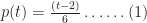
These two expressions are sometimes referred to as the probability distribution function (PDF). The PDF described by equations (1) and (2) is illustrated in Figure 1. (Note: Please click on the Figures to view full-size images)

Figure 1: Probability distribution for task

Now, a PDF tells us the probability that the task will finish at a particular time $t$ . However, we are more interested in knowing whether or not the task will be completed by time $t$ . – i.e. at or before time $t$ . This quantity, which we’ll denote by $P(t)$ (capital P), is sometimes known as the cumulative distribution function (CDF). The CDF is obtained by summing up the probabilities from $t=2$ hrs to time $t$ . It is not hard to show that the CDF for the task at hand is given by the following equations:

$P(t)=\frac{(t-2)^2}{12}\ldots\ldots(3)$ for 2 hours $\leq t \leq$ 4 hours

and,

$P(t)=1- \frac{(8-t)^2}{24}\ldots\ldots(4)$ for 4 hours $\leq t \leq$ 8 hours

For a detailed derivation, please see my introductory post. The CDF for the distribution is shown in Figure 2.

Figure 2: CDF for task

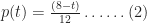
Now for the complicating factor: let us assume there is a risk that has a bearing on this task. The risk could be any known factor that has a negative impact on task duration. For example, it could be that a required resource is delayed or that the deliverable will fails a quality check and needs rework. The consequence of the risk – should it eventuate – is that the task takes longer. How much longer the task takes depends on specifics of the risk. For the purpose of this example we’ll assume that the additional time taken is also described by a triangular distribution with a minimum, most likely and maximum time of 1, 2 and 3 hrs respectively. The PDF $p_{r}(t)$ for the additional time taken due to the risk is:

$p_{r}(t)=(t-1)\dots\ldots(5)$ for 1 hour $\leq t \leq$ 2 hours

And

$p_{r}(t)=(3-t)\dots\ldots(6)$ for 2 hrs $\leq t \leq$ 3 hours

The figure for this distribution is shown in Figure 3.

Figure 3: Probability distribution of additional time due to risk

The CDF for the additional time taken if the risk eventuates (which we’ll denote by $P_{r}(t)$ ) is given by:

$P_{r}(t)=\frac{(t-1)^2}{2}\ldots\ldots(7)$ for 1 hour $\leq t \leq$ 2 hours

and,

$P_{r}(t)=1- \frac{(3-t)^2}{2}\ldots\ldots(8)$ for 2 hours $\leq t \leq$ 3 hours

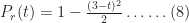
The CDF for the risk consequence is shown in Figure 4.

Figure 4: CDF of additional time due to risk

Before proceeding with the simulation it is worth clarifying what all this means, and what we want to do with it.

Firstly, equations 1-4 describe the inherent uncertainty associated with the task while equations 5 through 8 describe the consequences of the risk, if it eventuates.

Secondly, we have described the task and the risk separately. In reality, we need a unified description of the two – a combined distribution function for the uncertainty associated with the task and the risk taken together. This is what the simulation will give us.

Finally, one thing I have not yet specified is the probabilty that the risk will actually occur. Clearly, the higher the probability, the greater the potential delay. Below I carry out simulations for risk probabilities of varying from 0.1 to 0.5.

That completes the specification of the problem – let’s move on to the simulation.

The simulation

The simulation procedure I used for the zero-risk case (i.e. the task described by equations 1 and 2 ) is as follows :

Generate a random number between 0 and 1. Treat this number as the cumulative probability, $P(t)$ for the simulation run. [You can generate random numbers in Excel using the rand() function]
Find the time, $t$ , corresponding to $P(t)$ by solving equations (3) or (4) for $t$ . The resulting value of $t$ is the time taken to complete the task.
Repeat steps (1) and (2) for a sufficiently large number of trials.

The frequency distribution of completion times for the task, based on 30,000 trials is shown in Figure 5.

Figure 5: Simulation histogram for zero-risk case

As we might expect, Figure 5 can be translated to the probability distribution shown in Figure 1 by a straightforward normalization – i.e. by dividing each bar by the total number of trials.

What remains to be done is to incorporate the risk (as modeled in equations 5-6) into the simulation. To simulate the task with the risk, we simply do the following for each trial:

Simulate the task without the risk as described earlier.
Generate another random number between 0 and 1.
If the random number is less than the probability of the risk, then simulate the risk. Note that since the risk is described by a triangular function, the procedure to simulate it is the same as that for the task (albeit with different parameters).
If the random number is greater than the probability of the risk, do nothing.
Add the results of 1 and 4. This is the outcome of the trial.
Repeat steps 1-5 for as many trials as required.

I performed simulations for the task with risk probabilities of 10%, 30% and 50%. The frequency distributions of completion times for these are displayed in Figures 6-8 (in increasing order of probability). As one would expect, the spread of times increases with increasing probability. Further, the distribution takes on a distinct second peak as the probability increases: the first peak is at $t=4$ , corresponding to the most likely completion time of the risk-free task and the second at $t=6$ corresponding to the most likely additional time of 2 hrs if the risk eventuates.

Figure 6: Simulation histogram (10% probability of risk)

Figure 7: Simulation histogram (30% probability of risk)

Figure 8: Frequency histogram (50% probability of risk)

It is also instructive to compare average completion times for the four cases (zero-risk and 10%, 30% and 50%). The average can computed from the simulation by simply adding up the simulated completion times (for all trials) and dividing by the total number of simulation trials (30,000 in our case). On doing this, I get the following:

Average completion time for zero-risk case = 4.66 hr

Average completion time with 10% probability of risk = 4.89 hrs

Average completion time with 30% probability of risk = 5.36 hrs

Average completion time with 50% probability of risk= 5.83 hrs

No surprises here.

One point to note is that the result obtained from the simulation for the zero-risk case compares well with the exact formula for a triangular distribution (see the Wikipedia article for the triangular distribution):

$t_{av} = \frac{t_{worst}+t_{best}+t_{most likely}}{3}=\frac{8+2+4}{3}=4.67$ hrs

This serves as a sanity check on the simulation procedure.

It is also interesting to compare the cumulative probabilities of completion in the zero-risk and high risk (50% probability) case. The CDFs for the two are shown in Figure 9. The co-plotted CDFs allow for a quick comparison of completion time predictions. For example, in the zero-risk case, there is about a 90% chance that the task will be completed in a little over 6 hrs whereas when the probability of the risk is 50%, the 90% completion time increases to 8 hrs (see Figure 9).

Figure 9: CDFs for zero risk and 50% probability of risk cases

Next steps and wrap up

For those who want to learn more about simulating project uncertainty and risk, I can recommend the UK MOD paper – Three Point Estimates And Quantitative Risk Analysis A Process Guide For Risk Practitioners. The paper provides useful advice on how three point estimates for project variables should be constructed. It also has a good discussion of risk and how it should be combined with the inherent uncertainty associated with a variable. Indeed, the example I have described above was inspired by the paper’s discussion of uncertainty and risk.

Of course, as with any quantitative predictions of project variables, the numbers are only as reliable as the assumptions that go into them, the main assumption here being the three point estimates that were used to derive the distributions for the task uncertainty and risk (equations 1-2 and 5-6). Typically these are obtained from historical data. However, there are well known problems associated with history-based estimates. For one, as we can never be sure that the historical tasks are similar to the one at hand in ways that matter (this is the reference class problem). As Shim Marom warns us in this post, all our predictions depend on the credibility of our estimates. Quoting from his post:

Can you get credible three point estimates? Do you have access to credible historical data to support that? Do you have access to Subject Matter Experts (SMEs) who can assist in getting these credible estimates?

If not, don’t bother using Monte Carlo.

In closing, I hope my readers will find this simple example useful in understanding how uncertainty and risk can be accounted for using Monte Carlo simulations. In the end, though, one should always keep in mind that the use of sophisticated techniques does not magically render one immune to the GIGO principle.

Written by K

February 17, 2011 at 9:55 pm

Posted in Estimation, Monte Carlo Simulation, Probability, Project Management, Risk analysis, Statistics

Six ways in which project estimates go wrong

with 7 comments

Despite the increasing focus on project estimation, the activity still remains more guesswork than art or science. In his book on the fallacies of software engineering, Robert Glass has this to say about it:

Estimation, as you might imagine, is the process by which we determine how long a project will take and how much it will cost. We do estimation very badly in the software field. Most of our estimates are more like wishes than realistic targets. To make matters worse, we seem to have no idea how to improve on those very bad practices. And the result is, as everyone tries to meet an impossible estimation target, shortcuts are taken, good practices are skipped, and the inevitable schedule runaway becomes a technology runaway as well…

Moreover, he suggests that poor estimation is one of the top two causes of project failure.

Now, there are a number of reasons why project estimates go wrong, but in my experience there are half-dozen standouts. Here they are, in no particular order:

1. False analogies: Project estimates based on historical data are generally considered to be more reliable than those developed using other methods such as expert judgement (see this article, from the MS Project support site for example). This is fine and good as long as one uses data from historical projects that are identical to the one at hand in relevant ways. Problem is, one rarely knows what is relevant and what isn’t. It is all too easy too select a project that is superficially similar to the one at hand, but actually differs in critical ways. See my posts on false analogies and the reference class problem for more on this point.

2. False precision: Project estimates are often quoted as single numbers rather than ranges. Such estimates are incorrect because they ignore the fact that uncertain quantities should be quantified by a range of numbers (or more accurately, a distribution) rather than point values. As Dr. Sam Savage emphasises in his book, The Flaw of Averages: an uncertain quantity is a shape, not a number (see my review of the book for more on this point). In short, an estimate quoted as a single number is almost guaranteed to be incorrect.

3. Estimation by decree: It should be obvious that estimation must be done by those who will do the work. Unfortunately this principle is one of the first to be sacrificed on Death March Projects. In such projects, schedules are shoe-horned into predetermined timelines, with estimates cooked up by those who have little or no idea of the actual effort involved in doing the work.

4. Subjectivity: This is where estimates are plucked out of thin air and “justified” based on gut-feel and other subjective notions. Such estimates are prone to overconfidence and a range of other cognitive biases. See my post on cognitive biases as project meta-risks for a detailed discussion of how these biases manifest themselves in project estimates.

5. Coordination neglect: Projects consist of diverse tasks that need to be coordinated and integrated carefully. Unfortunately, the time and effort needed for coordination and integration is often underestimated (or even totally overlooked) by project decision makers. This is referred to as coordination neglect. Coordination neglect is a problem in projects of all sizes, but is generally more significant for projects involving large teams (see this paper for an empirical study of the effect of team size on coordination neglect). As one might imagine, coordination neglect also becomes a significant problem in projects that consist of a large number of dependent tasks or have a large number of external dependencies.

6. Too coarse grained: Large tasks are made up of smaller tasks strung together in specific ways. Consequently, estimates for large tasks should be built up from estimates for the smaller sub-tasks. . Teams often short-circuit the process by attempting to estimate the large task directly. Such estimates usually turn out to be incorrect because sub-tasks are overlooked. Another problem is coordination neglect between sub-tasks, as discussed in the earlier point. It is true – – the devil is always in the details.

I should emphasise that the above list based on personal experience, not on any systematic study.

I’ll conclude this piece with another fragment from Glass, who is not very optimistic about improvements in the area of project estimation. As he states in his book:

The bottom line is that, here in the first decade of the twenty-first century, we don’t know what constitutes a good estimation approach, one that can yield decent estimates with good confidence that they will really predict when a project will be completed and how much it will cost. That is a discouraging bottom line. Amidst all the clamor to avoid crunch mode and end death marches, it suggests that so long as faulty schedule and cost estimates are the chief management control factors on software projects, we will not see much improvement.

True enough, but being aware of the ways in which estimates can go wrong is the first step towards improving them.

Written by K

October 1, 2010 at 4:55 am

Posted in Bias, Corporate IT, Estimation, IT Management, Project Management, Risk analysis

Eight to Late

Archive for the ‘Estimation’ Category

The drunkard’s dartboard: an intuitive explanation of Monte Carlo methods