Archive for the ‘Estimation’ Category
The reference class problem and its implications for project management
Introduction
Managers make decisions based on incomplete information, so it is no surprise that the tools of probability and statistics have made their way into management practice. This trend has accelerated somewhat over the last few years, particularly with the availability of software tools that simplify much of the grunt-work of using probabilistic techniques such as Monte Carlo methods or Bayesian networks. Purveyors of tools and methodologies and assume probabilities (or more correctly, probability distributions) to be known, or exhort users to determine probabilities using relevant historical data. The word relevant is important: it emphasises that the data used to calculate probabilities (or distributions) should be from situations that are similar to the one at hand. This innocuous statement papers over a fundamental problem in the foundations of probability: the reference class problem. This post is a brief introduction to the reference class problem and its implications for project management.
I’ll begin with some background and then, after defining the problem, I’ll present a couple of illustrations of the problem drawn from project management.
Background and the Problem
The most commonly held interpretation of probability is that it is a measure of the frequency with which an event of interest occurs. In this frequentist view, as it is called, probability is defined as the ratio of the number of times the event of interest occurs to the total number of events. An example might help clarify what this means: the probability that a specific project will finish on time is given by the ratio of the number of similar projects that have finished on time to the total number of similar projects undertaken (including both on-time and not-on-time projects).
At first sight the frequentist approach seems a reasonable one. However, in this straightforward definition of probability lurks a problem: how do we determine which events are similar to the one at hand? In terms of the example: what are the criteria by which we can determine the projects that resemble the one we’re interested in? Do we look at projects with similar scope, or do we use size (in terms of budget, resources or other measure), or technology or….? There could be a range of criteria that one could use, but one never knows with certainty which one(s) is (are) the right one(s). Why is it an issue? It’s an issue because probability changes depending on the classification criteria used. This is the reference class problem.
In a paper entitled The Reference Class Problem is Your Problem Too, the philosopher Alan Hajek sums it up as follows:
The reference class problem arises when we want to assign a probability to a proposition (or sentence, or event) X, which may be classified in various ways, yet its probability can change depending on how it is classified.
Incidentally, in another paper entitled Conditional Probability is the Very Guide of Life, Hajek discusses how the reference class problem afflicts all major interpretations of probability, not just the frequentist approach. We’ll stick with the latter interpretation since it is the one used in project management practice and research… and virtually all the social and natural sciences to boot.
The reference class problem in project management
Let’s look at a couple of project management-related illustrations of the reference class problem.
First up, consider the technique of reference class forecasting which I’ve discussed in this post. Note that reference class forecasting technique is distinct from the reference class problem although, as we shall see in less than a minute, the technique is fatally afflicted by the problem.
What’s reference class forecasting? To quote from the post referenced earlier, the technique involves:
…creating a probability distribution of estimates based on data for completed projects that are similar to the one of interest, and then comparing the said project with the distribution in order to get a most likely outcome. Basically, [it] consists of the following steps:
- Collecting data for a number of similar past projects – these projects form the reference class. The reference class must encompass a sufficient number of projects to produce a meaningful statistical distribution, but individual projects must be similar to the project of interest.
- Establishing a probability distribution based on (reliable!) data for the reference class. The challenge here is to get good data for a sufficient number of reference class projects.
- Predicting most likely outcomes for the project of interest based on comparisons with the reference class distribution.
Now, the key assumption in reference class forecasting is that it is possible to identify a number of completed projects that are similar to the one at hand. But what does “similar” mean? Clearly the composition of the reference class depends on the similarity criteria used, and consequently so does the resulting distribution. Reference class forecasting is a victim of the reference class problem!
The reference class problem will affect any technique that uses arbitrary criteria to determine the set of all possible events. As another example, the probability distributions used in Monte Carlo simulations (of project cost, duration or whatever) are determined using historical data. Again, typically one selects projects (or tasks – if one is doing a task level simulation) that are similar to the one at hand. Defining “similar” is left to common sense or expert judgement or some other subjective approach. Yet, by the most commonly used definition, a project is a “temporary endeavor, having a defined beginning and end, undertaken to meet unique goals and objectives”. By definition, therefore, we never do the same project twice – at best we do the same project differently (and the same applies to tasks). So, despite ones best intentions and efforts, historical data can never be totally congruent to the situation at hand. There will always be differences, and one cannot tell with certainty that those differences do not matter.
Truth be told, most organizations do not retain data on completed projects – except superficial stuff that isn’t much use. The reference class problem seems to justify the position of this slack majority. After all, why bother keeping data when one isn’t able to use it to predict project performance. This argument is wrong-headed: although one cannot use it to calculate probabilities, historical data is useful because it keeps us from repeating our errors. Just don’t expect the data to yield reliable quantitative information on probabilities.
Before I close this piece, I should clarify that there are areas in which the reference class problem is not an issue. In physics, for example, the discipline of statistical mechanics is founded on the principle that the average motion of large collections of molecules can be treated statistically. Clearly, there is no problem here: molecules are indeed indistinguishable from each other, so it is clear that a particular molecule (of a gas in a container of carbon dioxide, say) belongs to the reference class of all carbon dioxide molecules in that container. In general this is true of any situation where one is dealing with a large collection of identical (or very similar) entities.
Conclusion
The reference class problem affects most probabilistic methods in project management and other areas of the social sciences. It is a problem because it is often impossible to know beforehand which attributes of the objects or events of interest are the most significant ones. Consequently it is impossible to determine with certainty whether or not a particular object or event belongs to a defined reference class.
I’ll end with an anecdote to illustrate my point:
Some time ago I was asked to provide estimates for design work that was superficially similar to something I’d done before. “You’ve done this before,” a manager said, “so you should be able to estimate this quite accurately.”
As many best practices and methodologies recommend, I used a mix of historical data and “expert” judgement (and added in a dash of padding) to arrive at (what I thought was) a robust estimate. To all you agilists out there, an incremental approach was not an option in this case.
I got it wrong – badly wrong. It turned out that the unique features of the project, which weren’t apparent at first, made a mockery of my estimates. I didn’t know it then, but I’d fallen victim to the reference class problem.
Finally, it should be clear that although my examples are project management focused, the arguments are quite general. They apply to all areas of management theory and practice, and indeed to most areas of inquiry that use probabilistic techniques. To use the words of Alan Hajek: the reference class problem is your problem too.
The Flaw of Averages – a book review
Introduction
I’ll begin with an example. Assume you’re having a dishwasher installed in your kitchen. This (simple?) task requires the services of a plumber and an electrician, and both of them need to be present to complete the job. You’ve asked them to come in at 7:30 am. Going from previous experience, these guys are punctual 50% of the time. What’s the probability that work will begin at 7:30 am?
At first sight, it seems there’s a 50% chance of starting on time. However, this is incorrect – the chance of starting on time is actually 25%, the product of the individual probabilities for each of the tradesmen. This simple example illustrates the central theme of a book by Sam Savage entitled, The Flaw of Averages: Why We Underestimate Risk in the Face of Uncertainty. This post is a detailed review of the book.
The key message that Savage conveys is that uncertain quantities cannot be represented by single numbers, rather they are a range of numbers each with a different probability of occurrence. Hence such quantities cannot be manipulated using standard arithmetic operations. The example mentioned in the previous paragraphs illustrate this point. This is well known to those who work with uncertain numbers (actuaries, for instance), but is not so well understood by business managers and decision makers. Hence the executive who asks his long-suffering subordinate to give him a projected sales figure for next month, with the quoted number then being taken as the 100% certain figure. Sadly such stories are more the norm than the exception, so it is clear that there is a need for a better understanding of how uncertain quantities should be interpreted. The main aim of the book is to help those with little or no statistical training achieve that understanding.
Developing an intuition for uncertainty
Early in the book, Savage presents five tools that can be used to develop a feel for uncertainty. He refers to these tools as mindles – or mind handles. His five mindles for uncertainty are:
- Risk is in the eye of the beholder, uncertainty isn’t. Basically this implies that uncertainty does not equate to risk. An uncertain event is a risk only if there is a potential loss or gain involved. See my review of Douglas Hubbard’s book on the failure of risk management for more on risk vs. uncertainty.
- An uncertain quantity is a shape (or a distribution of numbers) rather than a single number. The broadness of the shape is a measure of the degree of uncertainty. See my post on the inherent uncertainty of project task estimates for an intuitive discussion of how a task estimate is a shape rather than a number.
- A combination of several uncertain numbers is also a shape, but the combined shape is very different from those of the individual uncertainties. Specifically, if the uncertain quantities are independent, the combined shape can be narrower (i.e. less uncertain) than that of the individual shapes. This provides the justification for portfolio diversification, which tells us not to put all our money on one horse, or eggs in one basket etc. See my introductory post on Monte Carlo simulations to see an example of how multiple uncertain quantities can combine in different ways.
- If the individual uncertain quantities (discussed in the previous point) aren’t independent, the overall uncertainty can increase or decrease depending on whether the quantities are positively or negatively related. The nature of the relationship (positive or negative) can be determined from a scatter plot of the quantities. See my post on simulation of correlated project tasks for examples of scatter plots. The post also discusses how positive relationships (or correlations) can increase uncertainty.
- Plans based on average numbers are incorrect on average. Using average numbers in plans usually entails manipulating them algebraically and/or plugging them into functions. Savage explains how the form of the function can lead to an overestimation or underestimation of the planned value. Although this sounds a somewhat abstruse, the basic idea is simple: manipulating an average number using mathematical operations will amplify the error caused by the flaw of averages.
Savage explains the above concepts using simple arithmetic supplemented with examples drawn from a range of real-life business problems.
The two forms of the flaw of averages
The book makes a distinction between two forms of the flaw of averages. In its first avatar, the flaw states that the combined average of two uncertain quantities equals the sum of their individual averages, but the shape of the combined uncertainty can be very different from the sum of the individual shapes (Recall that an uncertain number is a shape, but its average is a number). Savage calls this the weak form of the flaw of averages. The weak form applies when one deals with uncertain quantities directly. An example of this is when one adds up probabilistic estimates for two independent project tasks with no lead or lag between them. In this case the average completion time is the sum of the average completion times for the individual tasks, but the shape of the distribution of the combined tasks does not resemble the shape of the individual distributions. The fact that the shape is different is a consequence of the fact that probabilities cannot be “added up” like simple numbers. See the first example in my post on Monte Carlo simulation of project tasks for an illustration of this point.
In contrast, when one deals with functions of uncertain quantities, the combined average of the functions does not equal the sum of the individual averages. This happens because functions “weight” random variables in a non-uniform manner, thereby amplifying certain values of the variable. An example of this is where we have two sequential tasks with an earliest possible start time for the second. The earliest possible start time for the second task introduces a nonlinearity in cases where the first task finishes early (essentially because there is a lag between the finish of the first task and the start of the second in this situation). The constraint causes the average of the combined tasks to be greater than the sum of the individual averages. Savage calls this the strong form of the flaw of averages. It applies whenever one deals with nonlinear functions of uncertain variables. See the second example in my post on Monte Carlo simulation of multiple project tasks for an illustration of this point.
Much of the book presents real-life illustrations of the two forms of the flaw in risk assessment, drawn from finance to the film industry and from petroleum to pharmaceutical supply chains. He also covers the average-based abuse of statistics in discussions on topical “hot-button” issues such as climate change and health care.
De-jargonising statistics
A layperson-friendly feature of the book is that it explains statistical terms in plain English. As an example, Savage spends an entire chapter demystifying the term correlation using scatter plots . Another term that he explains is the Central Limit Theorem (CLT), which states that the sum of independent random variables resembles the Normal (or bell-shaped) distribution. A consequence of CLT is that one can reduce investment risk by diversifying one’s investments – i.e. making several (small) independent investments rather than a single (large) one – this is essentially mindle # 3 discussed earlier.
Decisions, decisions
Towards the middle of the book, Savage makes a foray into decision theory, focusing on the concept of value of information. Since decisions are (or should be) made on the basis of information, one needs to gather pertinent information prior to making a decision. Now, information gathering costs money (and time, which translates to money). This brings up the question as to how much should one spend in collecting information relevant to a particular decision? It turns out that in many cases one can use decision theory to put a dollar value on a particular piece of information. Surprisingly it turns out that organisations often over-spend in gathering irrelevant information. Savage spends a few chapters discussing how one can compute the value of information based on simple techniques of decision theory. As interesting as this section is, however, I think it is a somewhat disconnected from the rest of the book.
Curing the flaw: SIPs, SLURPS and Probability Management
The last part of the book is dedicated to outlining a solution (or as Savage calls it, a cure) to average-based – or flawed – statistical thinking. The central idea is to use pre-generated libraries of simulation trials for variables of interest. Savage calls such a packaged set of simulation trials a Stochastic Information Packet (SIP). Here’s an example of how it might work in practice:
Most business organisations worry about next year’s sales. Different divisions in the organisation might forecast sales using different of techniques. Further, they may use these forecasts as the basis for other calculations (such as profit and expenses for example). The forecasted numbers cannot be compared with each other because each calculation is based on different simulations or worse, different probability distributions. The upshot of this is that forecasted sales results can’t be combined or even compared. The problem can be avoided if everyone in the organisation uses the same SIP for forecasted sales. The results of calculations can be compared, and even combined, because they are based on the same simulation.
Calculations that are based on the same SIP (or set of SIPs) form a set of simulations that can be combined and manipulated using arithmetic operations. Savage calls such sets of simulations, Scenario Library Units with Relationships Preserved (or SLURPS). The name reflects the fact that each of the calculations is based on the same set of sales scenarios (or results of simulation trials). Regarding the terminology: I’m not a fan of laboured acronyms, but concede that they can serve as a good mnemonics.
The proposed approach ensures that the results of the combined calculations will avoid the flaw of averages,and exhibit the correct statistical behaviour. However, it assumes that there is an organisation-wide authority responsible for generating and maintaining appropriate SIPs. This authority – the probability manager – will be responsible for a “database” of SIPs that covers all uncertain quantities of interest to the business, and make these available to everyone in the organisation who needs to use them. To quote from the book, probability management involves:
…a data management system in which the entities being managed are not numbers, but uncertainties, that is, probability distributions. The central database is a Scenario Library containing thousands of potential future values of uncertain business parameters. The library exchanges information with desktop distribution processors that do for probability distributions what word processors did for words and what spreadsheets did for numbers.
Savage sees probability management as a key step towards managing uncertainty and risk in a coherent manner across organisations. He mentions that some organizations that have already started down this route (Shell and Merck, for instance). The book can thus also be seen as a manifesto for the new discipline of probability management.
Conclusion
I have come across the flaw of averages in various walks of organizational life ranging from project scheduling to operational risk analysis. Most often, the folks responsible for analysing uncertainty are aware of the flaw, and have the requisite knowledge of statistics to deal with it. However, such analyses can be hard to explain to those who lack this knowledge. Hence managers who demand a single number. Yes, such attitudes betray a lack of understanding of what uncertain numbers are and how they can be combined, but that’s the way it is in most organizations. The book is directed largely to that audience.
To sum up: the book is an entertaining and informative read on some common misunderstandings of statistics. Along the way the author translates many statistical principles and terms from “jargonese” to plain English. The book deserves to be read widely, especially by those who need it the most: managers and other decision-makers who need to understand the arithmetic of uncertainty.
Trumped by conditionality: why many posts on this blog are not interesting
Introduction
A large number of the posts on this blog do not get much attention – not too many hits and few if any comments. There could be several reasons for this, but I need to consider the possibility that readers find many of the things I write about uninteresting. Now, this isn’t for the want of effort from my side: I put a fair bit of work into research and writing, so it is a little disappointing. However, I take heart from the possibility that it might not be entirely my fault: there’s a statistical reason (excuse?) for the dearth of quality posts on this blog. This (possibly uninteresting) post discusses this probabilistic excuse.
The argument I present uses the concepts of conditional probability and Bayes Theorem. Those unfamiliar with these may want to have a look at my post on Bayes theorem before proceeding further.
The argument
Grist for my blogging mill comes from a variety of sources: work, others’ stories, books, research papers and the Internet. Because of time constraints, I can write up only a fraction of the ideas that come to my attention. Let’s put a number to this fraction – say I can write up only 10% of the ideas I come across. Assuming that my intent is to write interesting stuff, this number corresponds to the best (or most interesting) ideas I encounter. Of course, the term “interesting” is subjective – an idea that fascinates me might not have the same effect on you. However this is a problem for most qualitative judgements, so we’ll accept this and move on.
If we denote the event “I have an interesting idea” by 


Then, if we denote the event “I have an idea that is uninteresting” by 

assuming that an idea must either be interesting or uninteresting (no other possibilities allowed).
Now, for me to write up an idea, I have to find it interesting (i.e. judge it as being in the top 10%). Let’s be generous and assume that I correctly recognise an interesting idea (as being interesting) 70% of the time. From this, the conditional probability of my writing a post given that I encounter an interesting idea, 

where 
On the flip side, let’s assume that I correctly recognise 80% of the uninteresting ideas that I encounter as being no good. This implies that I incorrectly identify 20% of the uninteresting stuff as being interesting. That is, 20% of the uninteresting stuff is wrongly identified as being blog-worthy. So, the conditional probability of my writing a post about an uninteresting idea, 

(If the above values for
Now, we want to figure out the probability that a post that appears on my blog is interesting – i.e. that a post is interesting given that I have written it up. Using the notation of conditional probability, this can be written as 
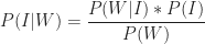

This can be written as,

Substituting this in the expression for Bayes Theorem, we get:

Using the numbers quoted above

So, only 28% of the ideas I write about are interesting. The main reason for is my inability to filter out all the dross. These “false positives” – which are all the ideas that I identify as interesting but are actually not – are represented by the 
So, there you go: it isn’t my fault really. 🙂
I should point out that the percentage of interesting ideas written up will be small whenever the false positive term is significant compared to the numerator. In this sense the result is insensitive to the values of the probabilities that I’ve used.
Of course, the argument presented above is based on a number of assumptions. I assume that:
- Mostreaders of this blog share my interests.
- The ideas that I encounter are either interesting or uninteresting.
- There is an arbitrary cutoff point between interesting and uninteresting ideas (the 10% cutoff).
- There is an objective criterion for what’s interesting and what’s not, and that I can tell one from the other 70% of the time.
- The relevant probabilities are known.
…and so, to conclude
I have to accept that much of the stuff I write about will be uninteresting, but can take consolation in the possibility that it is a consequence of conditional probabilities. I’m trumped by conditionality, once more.
Acknowledgements
This post was inspired by Peter Rousseeuw’s brilliant and entertaining paper entitled, Why the Wrong Papers Get Published. Thanks also go out to Vlado Bokan for interesting conversations about conditional probabilities and Bayes theorem.


