Estimation | Eight to Late

Archive for the ‘Estimation’ Category

An introduction to Monte Carlo simulation of project tasks

Introduction

In an essay on the uncertainty of project task estimates, I described how a task estimate corresponds to a probability distribution. Put simply, a task estimate is actually a range of possible completion times, each with a probability of occurrence specified by a distribution. If one knows the distribution, it is possible to answer questions such as: “What is the probability that the task will be completed within x days?”

The reliability of such predictions depends on how faithfully the distribution captures the actual spread of task durations – and therein lie at least a couple of problems. First, the probability distributions for task durations are generally hard to characterise because of the lack of reliable data (estimators are not very good at estimating, and historical data is usually not available). Second, many realistic distributions have complicated mathematical forms which can be hard to characterise and manipulate.

These problems are compounded by the fact that projects consist of several tasks, each one with its own duration estimate and (possibly complicated) distribution. The first issue is usually addressed by fitting distributions to point estimates (such as optimistic, pessimistic and most likely times as in PERT) and then refining these estimates and distributions as one gains experience. The second issue can be tackled by Monte Carlo techniques, which involve simulating the task a number of times (using an appropriate distribution) and then calculating expected completion times based on the results. My aim in this post is to present an example-based introduction to Monte Carlo simulation of project task durations.

Although my aim is to keep things reasonably simple (not too much beyond high-school maths and a basic understanding of probability), I’ll be covering a fair bit of ground. Given this, I’d best to start with a brief description of my approach so that my readers know what coming.

Monte Carlo simulation is an umbrella term that covers a range of approaches that use random sampling to simulate events that are described by known probability distributions. The first task then, is to specify the probability distribution. However, as mentioned earlier, this is generally unknown for task durations. For simplicity, I’ll assume that task duration uncertainty can be described accurately using a triangular probability distribution – a distribution that is particularly easy to handle from the mathematical point of view. The advantage of using the triangular distribution is that simulation results can be validated easily.

Using the triangular distribution isn’t a limitation because the method I describe can be applied to arbitrarily shaped distributions. More important, the technique can be used to simulate what happens when multiple tasks are strung together as in a project schedule (I’ll cover this in a future post). Finally, I’ll demonstrate a Monte Carlo simulation method as applied to a single task described by a triangular distribution. Although a simulation is overkill in this case (because questions regarding durations can be answered exactly without using a simulation), the example serves to illustrate the steps involved in simulating more complex cases – such as those comprising of more than one task and/or involving more complicated distributions.

So, without further ado, let me begin the journey by describing the triangular distribution.

The triangular distribution

Let’s assume that there’s a project task that needs doing, and the person who is going to do it reckons it will take between 2 and 8 hours to complete it, with a most likely completion time of 4 hours. How the estimator comes up with these numbers isn’t important at this stage – maybe there’s some guesswork, maybe some padding or maybe it is really based on experience (as it should be). What’s important is that we have three numbers corresponding to a minimum, most likely and maximum time. To keep the discussion general, we’ll call these $t_{min}$ , $t_{ml}$ and $t_{max}$ respectively, (we’ll get back to our estimator’s specific numbers later).

Now, what about the probabilities associated with each of these times?

Since $t_{min}$ and $t_{max}$ correspond to the minimum and maximum times, the probability associated with these is zero. Why? Because if it wasn’t zero, then there would be a non-zero probability of completion for a time less than $t_{min}$ or greater than $t_{max}$ – which isn’t possible [Note: this is a consequence of the assumption that the probability varies continuously – so if it takes on non-zero value, $p_{0}$ , at $t_{min}$ then it must take on a value slightly less than $p_{0}$ – but greater than 0 – at $t$ slightly smaller than $t_{min}$ ] . As far as the most likely time, $t_{ml}$ , is concerned: by definition, the probability attains its highest value at time $t_{ml}$ . So, assuming the probability can be described by a triangular function, the distribution must have the form shown in Figure 1 below.

Figure 1: Triangular Distribution

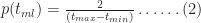
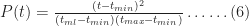
For the simulation, we need to know the equation describing the above distribution. Although Wikipedia will tell us the answer in a mouse-click, it is instructive to figure it out for ourselves. First, note that the area under the triangle must be equal to 1 because the task must finish at some time between $t_{min}$ and $t_{max}$ . As a consequence we have:

$\frac{1}{2}\times{base}\times{altitude}=\frac{1}{2}\times{(t_{max}-t_{min})}\times{p(t_{ml})}=1\ldots\ldots{(1)}$

where $p(t_{ml})$ is the probability corresponding to time $t_{ml}$ . With a bit of rearranging we get,

$p(t_{ml})=\frac{2}{(t_{max}-t_{min})}\ldots\ldots(2)$

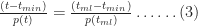
To derive the probability for any time $t$ lying between $t_{max}$ and $t_{ml}$ , we note that:

$\frac{(t-t_{min})}{p(t)}=\frac{(t_{ml}-t_{min})}{p(t_{ml})}\ldots\ldots(3)$

This is a consequence of the fact that the ratios on either side of equation (3) are equal to the slope of the line joining the points $(t_{min},0)$ and $(t_{ml}, p(t_{ml}))$ .

Figure 2

Substituting (2) in (3) and simplifying a bit, we obtain:

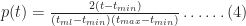
$p(t)=\frac{2(t-t_{min})}{(t_{ml}-t_{min})(t_{max}-t_{min})}\dots\ldots(4)$ for $t_{min}\leq t \leq t_{ml}$

In a similar fashion one can show that the probability for times lying between $t_{ml}$ and $t_{max}$ is given by:

$p(t)=\frac{2(t_{max}-t)}{(t_{max}-t_{ml})(t_{max}-t_{min})}\dots\ldots(5)$ for $t_{ml}\leq t \leq t_{max}$

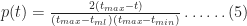
Equations 4 and 5 together describe the probability distribution function (or PDF) for all times between $t_{min}$ and $t_{max}$ .

Another quantity of interest is the cumulative distribution function (or CDF) which is the probability, $P$ , that the task is completed by a time $t$ . To reiterate, the PDF, $p(t)$ , is the probability of the task finishing at time $t$ whereas the CDF, $P(t)$ , is the probability of the task completing by time $t$ . The CDF, $P(t)$ , is essentially a sum of all probabilities between $t_{min}$ and $t$ . For $t < t_{min}$ this is the area under the triangle with apexes at ( $t_{min}$ , 0), (t, 0) and (t, p(t)). Using the formula for the area of a triangle (1/2 base times height) and equation (4) we get:

$P(t)=\frac{(t-t_{min})^2}{(t_{ml}-t_{min})(t_{max}-t_{min})}\ldots\ldots(6)$ for $t_{min}\leq t \leq t_{ml}$

Noting that for $t \geq t_{ml}$ , the area under the curve equals the total area minus the area enclosed by the triangle with base between t and $t_{max}$ , we have:

$P(t)=1- \frac{(t_{max}-t)^2}{(t_{max}-t_{ml})(t_{max}-t_{min})}\ldots\ldots(7)$ for $t_{ml}\leq t \leq t_{max}$

As expected, $P(t)$ starts out with a value 0 at $t_{min}$ and then increases monotonically, attaining a value of 1 at $t_{max}$ .

To end this section let's plug in the numbers quoted by our estimator at the start of this section: $t_{min}=2$ , $t_{ml}=4$ and $t_{max}=8$ . The resulting PDF and CDF are shown in figures 3 and 4.

Figure 3 - Triangular PDF (tmin=2, tml=4, tmax=8)

Figure 4 – Triangular CDF (tmin=2, tml=4, tmax=8)

Monte Carlo Simulation of a Single Task

OK, so now we get to the business end of this essay – the simulation. I’ll first outline the simulation procedure and then discuss results for the case of the task described in the previous section (triangular distribution with $t_{min}=2$ , $t_{ml}=4$ and $t_{max}=8$ ). Note that I used TK Solver – a mathematical package created by Universal Technical Systems – to do the simulations. TK Solver has built-in backsolving capability which is extremely helpful for solving some of the equations that come up in the simulation calculations. One could use Excel too, but my spreadsheet skills are not up to it :-(.

So, here’s my simulation procedure:

Generate a random number between 0 and 1. Treat this number as the cumulative probability, $P(t)$ for the simulation run. [Technical Note: I used the random number generator that comes with the TK Solver package (the algorithm used by the generator is described here). Excel’s random number generator is even better.]
Find the time, $t$ , corresponding to $P(t)$ by solving equations (6) or (7) for $t$ . The resulting value of $t$ is the time taken to complete the task. [Technical Note: Solving equation (6) or (7) for $t$ isn’t straightforward because $t$ appears in several places in the equations. One has two options to solve for $t$ a) Use numerical techniques such as the bisection or Newton-Raphson method or b) use the backsolve (goal seek) functionality in Excel or other mathematical packages. I used the backsolving capability of TK Solver to obtain t for each random value of P generated. TK Solver backsolves equations automatically – no fiddling around with numerical methods – which makes it an attractive option for these kinds of calculations.]
Repeat steps (1) and (2) N times, where N is a “sufficiently large” number – say 10,000.

I did the calculations for $N=10000$ using the triangular distribution with parameters $t_{min}=2$ , $t_{ml}=4$ and $t_{max}=8$ . This gave me 10,000 values of $P(t)$ and $t$ .

As an example of a simulation run proceeds, here’s the data from my first simulation run: the random number generator returned 0.490474700804856 (call it 0.4905). This is the value of $P(t)$ . The time corresponding to this cumulative probability is obtained by solving equation (7) numerically for $t$ . This gave $t = 4.503057452476027$ (call it 4.503) as shown in Figure 5. This is the completion time for the first run.

Figure 5

After completing 10,000 simulation runs, I sorted these into bins corresponding to time intervals of .25 hrs, starting from $t$ =2hrs through to $t$ =8 hrs. The resulting histogram is shown in Figure 6. Each bar corresponds to the number of simulation runs that fall within that time interval.

Figure 6: Distribution of simulation runs

As one might expect, this looks like the triangular distribution shown in Figure 4. There is a difference though: Figure 4 plots probability as a continuous function of time whereas Figure 6 plots the number of simulation runs as a step function of time. To convince ourselves that the two are really the same, lets look at the cumulative probability at $t_{ml}$ – i.e the probability that the task will be completed within 4 hrs. From equation 6 we get $P(t_{ml})=0.3333$ . The corresponding number from the simulation is simply the number of simulation runs that had a completion time less than or equal to 4 hrs, divided by the total number of simulation runs. For my simulation this comes out to be 0.3383. The agreement’s not perfect, but is convincing enough. Just to be sure, I performed the simulation a number of times – generating several sets of random numbers – and took the average of the predicted $P(t_{ml})$ . The agreement between theory and simulation improved, as expected.

Wrap up

A limitation of the triangular distribution is that it imposes an upper cut-off at $t_{max}$ . Long-tailed distributions may therefore be more realistic. In the end, though, the form distribution is neither here nor there because the technique can be applied to any distribution. The real question is: how do we obtain reliable distributions for our estimates? There’s no easy answer to this one, but one can start with three point estimates (as in PERT) and then fit these to a triangular (or more complicated) distribution. Although it is best if one has historical data, in the absence this one can always start with reasonable guesses. The point is to refine these through experience.

Another point worth mentioning is that simulations can be done at a level higher than that of an indivdual task. In their brilliant book – Waltzing With Bears: Managing Risk on Software Projects – De Marco and Lister demonstrate the use of Monte Carlo methods to simulate various aspects of project – velocity, time, cost etc. – at the project level (as opposed to the task level). I believe it is better to perform simulations at the lowest possible level (although it is a lot more work) – the main reason being that it is easier, and less error-prone, to estimate individual tasks than entire projects. Nevertheless, high level simulations can be very useful if one has reliable data to base these on.

I would be remiss if I didn’t mention some of the various Monte Carlo packages available in the market. I’ve never used any of these, but by all accounts they’re pretty good: see this commercial package or this one, for example. Both products use random number generators and sampling techniques that are far more sophisticated than the simple ones I’ve used in my example.

Finally, I have to admit that the example described in this post is a very complicated way of demonstrating the obvious – I started out with the triangular distribution and then got back the triangular distribution via simulation. My point, however, was to illustrate the method and show that it yields expected results in a situation where the answer is known. In a future post I’ll apply the method to more complex situations- for example, multiple tasks in series and parallel, with some dependency rules thrown in for good measure. Although, I’ll use the triangular distribution for individual tasks, the results will be far from obvious: simulation methods really start to shine as complexity increases. But all that will have to wait for later. For now, I hope my example has helped illustrate how Monte Carlo methods can be used to simulate project tasks.

Note added on 21 Sept 2009:

Follow-up to this article published here.

Note added on 14 Dec 2009:

See this post for a Monte Carlo simulation of correlated project tasks.

Written by K

September 11, 2009 at 11:05 pm

Posted in Estimation, Monte Carlo Simulation, portfolio management, Probability, Project Management, Statistics

Anchored and over-optimistic: why quick and dirty estimates are almost always incorrect

with 7 comments

Some time ago, a sales manager barged into my office. “I’m sorry for the short notice,” she said, “but you’ll need to make some modifications to the consolidated sales report by tomorrow evening.”

I could see she was stressed and I wanted to help, but there was an obvious question that needed to be asked. “What do you need done? I’ll have to get some details before I can tell you if it can be done within the time,” I replied.

She pulled up a chair and proceeded to explain what was needed. Within a minute or two I knew there was no way I could get it finished by the next day. I told her so.

“Oh no…this is really important. How long will it take?”

I thought about it for a minute or so. “OK how about I try to get it to you by day after?”

“Tomorrow would be better, but I can wait till day after.” She didn’t look very happy about it though. “Thanks,” she said and rushed away, not giving me a chance to reconsider my off-the-cuff estimate.

—

After she left, I had a closer look at what needed to be done. Soon I realised it would take me at least twice as long if I wanted to do it right. As it was, I’d have to work late to get it done in the agreed time, and may even have to cut a corner or two ( or three) in the process.

So why was I so wide off the mark?

I had been railroaded into giving the manager an unrealistic estimate without even realising it. When the manager quoted her timeline, my subconscious latched on to it as an initial value for my estimate. Although I revised the initial estimate upwards, I was “pressured” – albeit unknowingly – into quoting an estimate that was biased towards the timeline she’d mentioned. I was a victim of what psychologists call anchoring bias – a human tendency to base judgements on a single piece of information or data, ignoring all other relevant factors. In arriving at my estimate, I had focused on one piece of data (her timeline) to the exclusion of all other potentially significant information (the complexity of the task, other things on my plate etc.).

Anchoring bias was first described by Amos Tversky and Daniel Kahnemann in their pioneering paper entitled, Judgement under Uncertainty: Heuristics and Biases. Tversky and Kahnemann found that people often make quick judgements based on initial (or anchor) values that are suggested to them. As the incident above illustrates, the anchor value (the manager’s timeline) may have nothing to do with the point in question (how long it would actually take me to do the work). To be sure, folks generally adjust the anchor values based on other information. These adjustments, however, are generally inadequate. The final estimates arrived at are incorrect because they remain biased towards the initial value. As Tversky and Kahnemann state in their paper:

In many situations, people make estimates by starting from an initial value that is adjusted to yield the final answer. The initial value, or starting point, may be suggested by the formulation of the problem, or it may be the result of a partial computation. In either case, adjustments are typically insufficient. That is, different starting points yield different estimates, which are biased toward the initial values. We call this phenomenon anchoring.

Although the above quote may sound somewhat academic, be assured that anchoring is very real. It affects even day-to-day decisions that people make. For example, in this paper Neil Stewart presents evidence that credit card holders repay their debt more slowly when their statements suggest a minimum payment. In other words the minimum payment works as an anchor, causing the card holder to pay a smaller amount than they would have been prepared to (in the absence of an anchor).

Anchoring, however, is only part of the story. Things get much worse for complex tasks because another bias comes into play. Tversky and Kahnemann found that subjects tended to be over optimistic when asked to make predictions regarding complex matters. Again, quoting from their paper:

Biases in the evaluation of compound events are particularly significant in the context of planning. The successful completion of an undertaking, such as the development of a new product, typically has a conjunctive character: for the undertaking to succeed, each of a series of events must occur. Even when each of these events is very likely, the overall probability of success can be quite low if the number of events is large. The general tendency to overestimate the probability of conjunctive events leads to unwarranted optimism in the evaluation of the likelihood that a plan will succeed or that a project will be completed on time.

Such over-optimism in the face of complex tasks is sometimes referred to as the planning fallacy.¹

Of course, as discussed by Kahnemann and Fredrick in this paper, biases such as anchoring and the planning fallacy can be avoided by a careful, reflective approach to estimation – as opposed to a “quick and dirty” or intuitive one. Basically, a reflective approach seeks to eliminate bias by reducing the effect of individual judgements. This is why project management texts advise us (among other things) to:

Base estimates on historical data for similar tasks. This is the basis of reference class forecasting which I have written about in an earlier post.
Draft independent experts to do the estimation.
Use multipoint estimates (best and worst case scenarios)

In big-bang approaches to project management, one has to make a conscious effort to eliminate bias because there are fewer chances to get it right. On the other hand, iterative / incremental methodologies have bias elimination built-in because one starts with initial estimates, which include inaccuracies due to bias, and subsequently refine these as one progresses. The estimates get better as one goes along because every refinement is based on an improved knowledge of the task.

Anchoring and the planning fallacy are examples cognitive biases – patterns of deviations of judgement that humans display in a variety of situations. Since the pioneering work of Tversky and Kahnemann, these biases have been widely studied by psychologists. It is important to note that these biases come into play whenever quick and dirty judgements are involved. They occur even when subjects are motivated to make accurate judgements. As Tversky and Kahnemann state towards the end of their paper:

These biases are not attributable to motivational effects such as wishful thinking or the distortion of judgments by payoffs and penalties. Indeed, several of the severe errors of judgment reported earlier (in the paper) occurred despite the fact that subjects were encouraged to be accurate and were rewarded for the correct answers.

The only way to avoid cognitive biases in estimating is to proceed with care and consideration. Yes, that’s a time consuming, effort-laden process, but that’s the price one pays for doing it right. To paraphrase Euclid, there is no royal road to estimation.

Footnotes:

¹ The planning fallacy is related to optimism bias which I have discussed in my post on reference class forecasting.

Written by K

January 30, 2009 at 11:11 pm

Posted in Bias, Estimation, Project Management

Tagged with Estimating

A pert myth

with 5 comments

PERT (Program Evaluation and Review Technique) is a stock standard method to manage project schedule risk. It is taught (or at least mentioned) in just about every project management course. PERT was first used (and is considered to have originated) in the Polaris project, and is often credited as being one of the main reasons for the the success of that endeavour. The truth is considerably more nuanced: it turns out that PERT was used on the Polaris project more as PR than PM. It was often applied “after the fact” – when generating reports for Congress, who held the project purse-strings. This post is a brief look into the PERT myth, based on sources available online.

An excellent place to start is Glen Alleman’s post from 2005 entitled, Origins and Myth of PERT ¹. Glen draws attention to a RAND Corporation publication entitled, Quantitative Risk Analysis for Project Management – A Critical Review, written by Lionel Galway. The paper is essentially a survey of quantitative risk management and analysis techniques. The author has this to say about PERT:

…PERT was a great success from a public relations point of view, although only a relatively small portion of the Polaris program was ever managed using the technique. And this success led to adaptations of PERT such as PERT/cost that attempted to address cost issues as well. While PERT was widely acclaimed by the business and defense communities in the 1960s, later studies raised doubts about whether PERT contributed much to the management success of the Polaris project. Many contended that its primary contribution was to deflect management interference by the Navy and DoD (Department of Defense) by providing a “cover” of disciplined, quantitative, management carried out by modern methodologies…

Then, in the conclusion of the paper, he states:

…While the Polaris program touted PERT as a breakthrough in project management, as noted above not even a majority of the tasks in the project were controlled with PERT. Klementowski’s thesis in the late 1970s, although limited for generalization by the sampling technique, showed less than a majority of organizations using CPM/PERT techniques. And the interviews conducted for this report revealed a similar ambivalence: respondents affirmed the usefulness of the techniques in general, but did not provide much in the way of particular examples…

In a footnote on page 10 of the paper, the author draws attention to Sapolsky’s book The Polaris System Development: Bureaucratic and Programmatic Success in Government. Among other things, the book describes how the use of PERT on the project has been grossly overstated. Unfortunately the book is out of print, but there is an excellent review of it on Cadmus. The review has this to say about the use of PERT on the Polaris project:

…SPO (Special Projects Office) Director Vice Admiral William F. Raborn pushed PERT mercilessly. The colorful PERT charts impressed everyone, and coupled with the nature of the project, they exuded management “sex appeal.” This kept other DoD poachers at bay and politicians off SPO’s back. Other government services became so enamored with PERT, they quickly made it a requirement in subsequent contracts.A more objective assessment of PERT is that the network analysis² is the major benefit. PERT can reduce cost and time overruns, and make its practitioners look like better managers…

The Royal Navy knew of the over-inflated success of PERT when it embarked on its own Polaris program in the 1960’s. The Royal Navy deliberately adopted PERT, essentially to keep Whitehall, Parliament and other critics away from their project. It worked just as well for the RN as it did for the USN
…

I found the accounts of PERT presented in these sources fascinating, because they highlight how project management history can be so much more ambiguous (and messier) than textbooks, teachers and trainers would have us believe. Techniques are often taught without any regard to their origins and limitations. Thus disassociated from their origins, they take on a life of their own leading to myths where from it is difficult to separate fact from fiction.

Footnotes:

¹ Glen Alleman also discusses some limitations of PERT in this and another post on his blog.

² Network analysis refers to task sequencing (precedence and dependencies) rather than task durations.

Written by K

August 2, 2008 at 9:44 am

Posted in Estimation, Project Management

Eight to Late

Archive for the ‘Estimation’ Category

An introduction to Monte Carlo simulation of project tasks

Introduction

The triangular distribution

Monte Carlo Simulation of a Single Task

Wrap up

Anchored and over-optimistic: why quick and dirty estimates are almost always incorrect

A pert myth

Subscribe

Search

Author

Copyright

My book

Top Posts & Pages

Recent Posts

Categories

Archives

Blogroll

Other links

Eight to Late

Archive for the ‘Estimation’ Category

An introduction to Monte Carlo simulation of project tasks

Introduction

The triangular distribution

Monte Carlo Simulation of a Single Task

Wrap up

Rate this:

Share this:

Anchored and over-optimistic: why quick and dirty estimates are almost always incorrect

Rate this:

Share this:

A pert myth

Rate this:

Share this:

Subscribe

Search

Author

Copyright

My book

Top Posts & Pages

Recent Posts

Categories

Archives

Blogroll

Other links