Archive for the ‘Probability’ Category
The improbability of success
Anyone who has tidied up after a toddler intuitively understands that making a mess is far easier than creating order. The fundamental reason for this is that the number of messy states in the universe (or a toddler’s room) far outnumbers the ordered ones. As this point might not be obvious, I’ll demonstrate it via a simple thought experiment involving marbles:
Throw three marbles onto a flat surface. When the marbles come to rest, you are most likely to end up with a random configuration as in Figure 1.

Figure 1: A random configuration of 3 marbles
Indeed, you’d be extremely surprised if the three ended up being collinear as in Figure 2. Note that Figure 2 is just one example of many collinear possibilities, but the point I’m making is that if the marbles are thrown randomly, they are more likely to end up in a random state than a lined-up one.

Figure 2: an unlikely (ordered) configuration
This raises a couple of questions:
Question: On what basis can one claim that the collinear configuration is tidier or more ordered than the non-collinear one?
Naive answer: It looks more ordered. Yes, tidiness is in the eye of the beholder so it is necessarily subjective. However, I’ll wager that if one took a poll, an overwhelming number of people would say that the configuration in Figure 2 is more ordered than the one in Figure 1.
More sophisticated answer : The “state” of collinear marbles can be described using 2 parameters, the slope and intercept of the straight line that three marbles lie on (in any coordinate system) whereas the description of the nonlinear state requires 3 parameters. The first state is tidier because it requires fewer parameters. Another way to think about is that the line can be described by two marbles; the third one is redundant as far as the description of the state is concerned.
Question: Why is a tidier configuration less likely than a messy one?
Answer: May be you see this intuitively and need no proof, but here’s one just in case. Imagine rolling the three marbles one after the other. The first two, regardless of where they end up, will necessarily lie along a line (two points lie on the straight line joining them). Now, I think it is easy to see that if we throw the third marble randomly, it is highly unlikely end up on that line. Indeed, for the third marble to end up exactly on the same straight line requires a coincidence of near cosmic proportions.
I know, I know, this is not a proof, but I trust it makes the point.
Now, although it is near impossible to get to a collinear end state via random throws, it is possible to approximate it by changing the way we throw the marbles. Here’s how:
- Throw the marbles consecutively rather than in one go.
- When throwing the third marble, adjust its initial speed and direction in a way that takes into account the positions of the two marbles that are already on the surface. Remember these two already define a straight line.
The third throw is no longer random because it is designed to maximise the chance that the last marble will get as close as possible to the straight line defined by the first two. Done right, you’ll end up with something closer to the configuration in Figure 3 rather than the one in Figure 2.

Figure 3: an “approximately ordered” state
Now you’re probably wondering what this has to do with success. I’ll make the connection via an example that will be familiar to many readers of this blog: an organisation’s strategy. However, as I will reiterate later, the arguments I present are very general and can be applied to just about any initiative or situation.
Typically, a strategy sets out goals for an organisation and a plan to achieve them in a specified timeframe. The goals define a number of desirable outcomes, or states which, by design, are constrained to belong to a (very) small subset of all possible states the organisation can end up in. In direct analogy with the simple model discussed above it is clear that, left to its own devices, the organisation is more likely to end up in one of the much overwhelmingly larger number of “failed states” than one of the successful ones. Notwithstanding the popular quote about there being many roads to success, in reality there are a great many more roads to failure.
Of course, that’s precisely why organisations are never “left to their own devices.” Indeed, a strategic plan specifies actions that are intended to make a successful state more likely than an unsuccessful one. However, no plan can guarantee success; it can, at best, make it more likely. As in the marble game, success is ultimately a matter of chance, even when we take actions to make it more likely.
If we accept this, the key question becomes: how can one design a strategy that improves the odds of success? The marble analogy suggests a way to do this is to:
- Define success in terms of an end state that is a natural extension of your current state.
- Devise a plan to (approximately) achieve that end state. Such a plan will necessarily build on the current state rather than change it wholesale. Successful change is an evolutionary process rather than a revolutionary one.
My contention is that these points are often ignored by management strategists. More often than not, they will define an end state based on a textbook idealisation, consulting model or (horror!) best practice. The marble analogy shows why copying others is unlikely to succeed.
Figure 4 shows a variant of the marble game in which we have two sets of marbles (or organisations!), one blue, as before, and the other red.

Figure 4: Two distinct configurations of marbles (or organisations)
Now, it is considerably harder to align an additional marble with both sets of marbles than the blue one alone. Here’s why…
To align with both sets, the new marble has to end up close to the point that lies at the intersection of the blue and red lines in Figure 5. In contrast, to align with the blue set alone, all that’s needed is for it to get close to any point on the blue line.
QED!

Figure 5: Why copying others is not a good idea (see text for explanation)
Finally, on a broader note, it should be clear that the arguments made above go beyond organisational strategies. They apply to pretty much any planned action, whether at work or in one’s personal life.
So, to sum up: when developing an organisational (or personal) strategy, the first step is to understand where you are and then identify the minimal actions you need to take in order to get to an “improved” state that is consistent with your current one. Yes, this is akin to the incremental and evolutionary approach that Agilistas and Leaners have been banging on about for years. However, their prescriptions focus on specific areas: software development and process improvement. My point is that the basic principles are way broader because they are a direct consequence of a fundamental fact regarding the relative likelihood of order and disorder in a toddler’s room, an organisation, or even the universe at large.
A gentle introduction to Naïve Bayes classification using R
Preamble
One of the key problems of predictive analytics is to classify entities or events based on a knowledge of their attributes. An example: one might want to classify customers into two categories, say, ‘High Value’ or ‘Low Value,’ based on a knowledge of their buying patterns. Another example: to figure out the party allegiances of representatives based on their voting records. And yet another: to predict the species a particular plant or animal specimen based on a list of its characteristics. Incidentally, if you haven’t been there already, it is worth having a look at Kaggle to get an idea of some of the real world classification problems that people tackle using techniques of predictive analytics.
Given the importance of classification-related problems, it is no surprise that analytics tools offer a range of options. My favourite (free!) tool, R, is no exception: it has a plethora of state of the art packages designed to handle a wide range of problems. One of the problems with this diversity of choice is that it is often confusing for beginners to figure out which one to use in a particular situation. Over the next several months, I intend to write up tutorial articles covering many of the common algorithms, with a particular focus on their strengths and weaknesses; explaining where they work well and where they don’t. I’ll kick-off this undertaking with a simple yet surprisingly effective algorithm – the Naïve Bayes classifier.
Just enough theory
I’m going to assume you have R and RStudio installed on your computer. If you need help with this, please follow the instructions here.
To introduce the Naive Bayes algorithm, I will use the HouseVotes84 dataset, which contains US congressional voting records for 1984. The data set is in the mlbench package which is not part of the base R installation. You will therefore need to install it if you don’t have it already. Package installation is a breeze in RStudio – just go to Tools > Install Packages and follow the prompts.
The HouseVotes84 dataset describes how 435 representatives voted – yes (y), no (n) or unknown (NA) – on 16 key issues presented to Congress. The dataset also provides the party affiliation of each representative – democrat or republican.
Let’s begin by exploring the dataset. To do this, we load mlbench, fetch the dataset and get some summary stats on it. (Note: a complete listing of the code in this article can be found here)
It is good to begin by exploring the data visually. To this end, let’s do some bar plots using the basic graphic capabilities of R:
The plots are shown in Figures 1 through 3.

Fig 1: y and n votes for issue 1

Fig 2: Republican votes for issue 1.
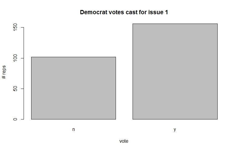
Fig 3: Democrat votes for issue 1.
Among other things, such plots give us a feel for the probabilities associated with how representatives from parties tend to vote on specific issues.
The classification problem at hand is to figure out the party affiliation from a knowledge of voting patterns. For simplicity let us assume that there are only 3 issues voted on instead of the 16 in the actual dataset. In concrete terms we wish to answer the question, “what is the probability that a representative is, say, a democrat (D) given that he or she has voted, say, 
In the notation of conditional probability this can be written as,

(Note: If you need a refresher on conditional probability, check out this post for a simple explanation.)
By Bayes theorem, which I’ve explained at length in this post, this can be recast as,

We’re interested only in relative probabilities of the representative being a democrat or republican because the predicted party affiliation depends only on which of the two probabilities is larger (the actual value of the probability is not important). This being the case, we can factor out any terms that are constant. As it happens, the denominator of the above equation – the probability of a particular voting pattern – is a constant because it depends on the total number of representatives (from both parties) who voted a particular way.
Now, using the chain rule of conditional probability, we can rewrite the numerator as:


Basically, the second term on the left hand side, 
Another application of the chain rule gives:

Where we have now factored out the n vote on the second issue.
The key assumption of Naïve Bayes is that the conditional probability of each feature given the class is independent of all other features. In mathematical terms this means that,

and

The quantity of interest, the numerator of equation (1) can then be written as:

The assumption of independent conditional probabilities is a drastic one. What it is saying is that the features are completely independent of each other. This is clearly not the case in the situation above: how representatives vote on a particular issue is coloured by their beliefs and values. For example, the conditional probability of voting patterns on socially progressive issues are definitely not independent of each other. However, as we shall see in the next section, the Naïve Bayes assumption works well for this problem as it does in many other situations where we know upfront that it is grossly incorrect.
Another good example of the unreasonable efficacy of Naive Bayes is in spam filtering. In the case of spam, the features are individual words in an email. It is clear that certain word combinations tend to show up consistently in spam – for example, “online”, “meds”, “Viagra” and “pharmacy.” In other words, we know upfront that their occurrences are definitely not independent of each other. Nevertheless, Naïve Bayes based spam detectors which assume mutual independence of features do remarkably well in distinguishing spam from ham.
Why is this so?
To explain why, I return to a point I mentioned earlier: to figure out the affiliation associated with a particular voting pattern (say, v1=y, v2=n,v3=y) one only needs to know which of the two probabilities 

This hints as to why the independence assumption might not be so quite so idiotic. Since the prediction depends only the on the maximum, the algorithm will get it right even if there are dependencies between feature providing the dependencies do not change which class has the maximum probability (once again, note that only the maximal class is important here, not the value of the maximum).
Yet another reason for the surprising success of Naïve Bayes is that dependencies often cancel out across a large set of features. But, of course, there is no guarantee that this will always happen.
In general, Naïve Bayes algorithms work better for problems in which the dependent (predicted) variable is discrete, even when there are dependencies between features (spam detection is a good example). They work less well for regression problems – i.e those in which predicted variables are continuous.
I hope the above has given you an intuitive feel for how Naïve Bayes algorithms work. I don’t know about you, but my head’s definitely spinning after writing out all that mathematical notation.
It’s time to clear our heads by doing some computation.
Naïve Bayes in action
There are a couple of well-known implementations of Naïve Bayes in R. One of them is the naiveBayes method in the e1071 package and the other is NaiveBayes method in the klaR package. I’ll use the former for no other reason than it seems to be more popular. That said, I have used the latter too and can confirm that it works just as well.
We’ve already loaded and explored the HouseVotes84 dataset. One of the things you may have noticed when summarising the data is that there are a fair number of NA values. Naïve Bayes algorithms typically handle NA values either by ignoring records that contain any NA values or by ignoring just the NA values. These choices are indicated by the value of the variable na.action in the naiveBayes algorithm, which is set to na.omit (to ignore the record) or na.pass (to ignore the value).
Just for fun, we’ll take a different approach. We’ll impute NA values for a given issue and party by looking at how other representatives from the same party voted on the issue. This is very much in keeping with the Bayesian spirit: we infer unknowns based on a justifiable belief – that is, belief based on the evidence.
To do this I write two functions: one to compute the number of NA values for a given issue (vote) and class (party affiliation), and the other to calculate the fraction of yes votes for a given issue (column) and class (party affiliation).
sum_y<-sum(HouseVotes84[,col]==’y’ & HouseVotes84$Class==cls,na.rm = TRUE)
sum_n<-sum(HouseVotes84[,col]==’n’ & HouseVotes84$Class==cls,na.rm = TRUE)
return(sum_y/(sum_y+sum_n))}
Before proceeding, you might want to go back to the data and convince yourself that these values are sensible.
We can now impute the NA values based on the above. We do this by randomly assigning values ( y or n) to NAs, based on the proportion of members of a party who have voted y or n. In practice, we do this by invoking the uniform distribution and setting an NA value to y if the random number returned is less than the probability of a yes vote and to n otherwise. This is not as complicated as it sounds; you should be able to figure the logic out from the code below.
if(sum(is.na(HouseVotes84[,i])>0)) {
c1 <- which(is.na(HouseVotes84[,i])& HouseVotes84$Class==’democrat’,arr.ind = TRUE)
c2 <- which(is.na(HouseVotes84[,i])& HouseVotes84$Class==’republican’,arr.ind = TRUE)
HouseVotes84[c1,i] <-
ifelse(runif(na_by_col_class(i,’democrat’))<p_y_col_class(i,’democrat’),’y’,’n’)
HouseVotes84[c2,i] <-
ifelse(runif(na_by_col_class(i,’republican’))<p_y_col_class(i,’republican’),’y’,’n’)}
Note that the which function filters indices by the criteria specified in the arguments and ifelse is a vectorised conditional function which enables us to apply logical criteria to multiple elements of a vector.
At this point it is a good idea to check that the NAs in each column have been set according to the voting patterns of non-NAs for a given party. You can use the p_y_col_class() function to check that the new probabilities are close to the old ones. You might want to do this before you proceed any further.
The next step is to divide the available data into training and test datasets. The former will be used to train the algorithm and produce a predictive model. The effectiveness of the model will then be tested using the test dataset. There is a great deal of science and art behind the creation of training and testing datasets. An important consideration is that both sets must contain records that are representative of the entire dataset. This can be difficult to do, especially when data is scarce and there are predictors that do not vary too much…or vary wildly for that matter. On the other hand, problems can also arise when there are redundant predictors. Indeed, the much of the art of successful prediction lies in figuring out which predictors are likely to lead to better predictions, an area known as feature selection. However, that’s a topic for another time. Our current dataset does not suffer from any of these complications so we’ll simply divide the it in an 80/20 proportion, assigning the larger number of records to the training set.
Now we’re finally good to build our Naive Bayes model (machine learning folks call this model training rather than model building – and I have to admit, it does sound a lot cooler).
The code to train the model is anticlimactically simple:
Here we’ve invokedthe naiveBayes method from the e1071 package. The first argument uses R’s formula notation.In this notation, the dependent variable (to be predicted) appears on the left hand side of the ~ and the independent variables (predictors or features) are on the right hand side. The dot (.) is simply shorthand for “all variable other than the dependent one.” The second argument is the dataframe that contains the training data. Check out the documentation for the other arguments of naiveBayes; it will take me too far afield to cover them here. Incidentally, you can take a look at the model using the summary() or str() functions, or even just entering the model name in the R console:
Note that I’ve suppressed the output above.
Now that we have a model, we can do some predicting. We do this by feeding our test data into our model and comparing the predicted party affiliations with the known ones. The latter is done via the wonderfully named confusion matrix – a table in which true and predicted values for each of the predicted classes are displayed in a matrix format. This again is just a couple of lines of code:
| pred true | democrat | republican |
| democrat | 38 | 3 |
| republican | 5 | 22 |
The numbers you get will be different because your training/test sets are almost certainly different from mine.
In the confusion matrix (as defined above), the true values are in columns and the predicted values in rows. So, the algorithm has correctly classified 38 out of 43 (i.e. 38+5) Democrats and 22 out of 25 Republicans (i.e. 22+3). That’s pretty decent. However, we need to keep in mind that this could well be quirk of the choice of dataset. To address this, we should get a numerical measure of the efficacy of the algorithm and for different training and testing datasets. A simple measure of efficacy would be the fraction of predictions that the algorithm gets right. For the training/testing set above, this is simply 60/68 (see the confusion matrix above). The simplest way to calculate this in R is:
A natural question to ask at this point is: how good is this prediction. This question cannot be answered with only a single run of the model; we need to do many runs and look at the spread of the results. To do this, we’ll create a function which takes the number of times the model should be run and the training fraction as inputs and spits out a vector containing the proportion of correct predictions for each run. Here’s the function
I’ve not commented the above code as it is essentially a repeat of the steps described earlier. Also, note that I have not made any effort to make the code generic or efficient.
Let’s do 20 runs with the same training fraction (0.8) as before:
[9] 0.9102564 0.9080460 0.9139785 0.9200000 0.9090909 0.9239130 0.9605263 0.9333333
[17] 0.9052632 0.8977273 0.9642857 0.8518519
0.8519 0.9074 0.9170 0.9177 0.9310 0.9643
We see that the outcome of the runs are quite close together, in the 0.85 to 0.95 range with a standard deviation of 0.025. This tells us that Naive Bayes does a pretty decent job with this data.
Wrapping up
I originally intended to cover a few more case studies in this post, a couple of which highlight the shortcomings of the Naive Bayes algorithm. However, I realize that doing so would make this post unreasonably long, so I’ll stop here with a few closing remarks, and a promise to write up the rest of the story in a subsequent post.
To sum up: I have illustrated the use of a popular Naive Bayes implementation in R and attempted to convey an intuition for how the algorithm works. As we have seen, the algorithm works quite well in the example case, despite the violation of the assumption of independent conditional probabilities.
The reason for the unreasonable effectiveness of the algorithm is two-fold. Firstly, the algorithm picks the predicted class based on the largest predicted probability, so ordering is more important than the actual value of the probability. Secondly, in many cases, a bias one way for a particular vote may well be counteracted by a bias the other way for another vote. That is, biases tend to cancel out, particularly if there are a large number of features.
That said, there are many cases in which the algorithm fails miserably – and we’ll look at some of these in a future post. However, despite its well known shortcomings, Naive Bayes is often the first port of call in prediction problems simply because it is easy to set up and is fast compared to many of the iterative algorithms we will explore later in this series of articles.
Endnote
Thanks for reading! If you liked this piece, you might enjoy the other articles in my “Gentle introduction to analytics using R” series. Here are the links:
A gentle introduction to text mining using R
Three types of uncertainty you (probably) overlook
Introduction – uncertainty and decision-making
Managing uncertainty – deciding what to do in the absence of reliable information – is a significant part of project management and many other managerial roles. When put this way, it is clear that managing uncertainty is primarily a decision-making problem. Indeed, as I will discuss shortly, the main difficulties associated with decision-making are related to specific types of uncertainties that we tend to overlook.
Let’s begin by looking at the standard approach to decision-making, which goes as follows:
- Define the decision problem.
- Identify options.
- Develop criteria for rating options.
- Evaluate options against criteria.
- Select the top rated option.
As I have pointed out in this post, the above process is too simplistic for some of the complex, multifaceted decisions that we face in life and at work (switching jobs, buying a house or starting a business venture, for example). In such cases:
- It may be difficult to identify all options.
- It is often impossible to rate options meaningfully because of information asymmetry – we know more about some options than others. For example, when choosing whether or not to switch jobs, we know more about our current situation than the new one.
- Even when ratings are possible, different people will rate options differently – i.e. different people invariably have different preferences for a given outcome. This makes it difficult to reach a consensus.
Regular readers of this blog will know that the points listed above are characteristics of wicked problems. It is fair to say that in recent years, a general awareness of the ubiquity of wicked problems has led to an appreciation of the limits of classical decision theory. (That said, it should be noted that academics have been aware of this for a long time: Horst Rittel’s classic paper on the dilemmas of planning, written in 1973, is a good example. And there are many others that predate it.)
In this post I look into some hard-to-tackle aspects of uncertainty by focusing on the aforementioned shortcomings of classical decision theory. My discussion draws on a paper by Richard Bradley and Mareile Drechsler.
This article is organised as follows: I first present an overview of the standard approach to dealing with uncertainty and discuss its limitations. Following this, I elaborate on three types of uncertainty that are discussed in the paper.
Background – the standard view of uncertainty
The standard approach to tackling uncertainty was articulated by Leonard Savage in his classic text, Foundations of Statistics. Savage’s approach can be summarized as follows:
- Figure out all possible states (outcomes)
- Enumerate actions that are possible
- Figure out the consequences of actions for all possible states.
- Attach a value (aka preference) to each consequence
- Select the course of action that maximizes value (based on an appropriately defined measure, making sure to factor in the likelihood of achieving the desired consequence)
(Note the close parallels between this process and the standard approach to decision-making outlined earlier.)
To keep things concrete it is useful to see how this process would work in a simple real-life example. Bradley and Drechsler quote the following example from Savage’s book that does just that:
…[consider] someone who is cooking an omelet and has already broken five good eggs into a bowl, but is uncertain whether the sixth egg is good or rotten. In deciding whether to break the sixth egg into the bowl containing the first five eggs, to break it into a separate saucer, or to throw it away, the only question this agent has to grapple with is whether the last egg is good or rotten, for she knows both what the consequence of breaking the egg is in each eventuality and how desirable each consequence is. And in general it would seem that for Savage once the agent has settled the question of how probable each state of the world is, she can determine what to do simply by averaging the utilities (Note: utility is basically a mathematical expression of preference or value) of each action’s consequences by the probabilities of the states of the world in which they are realised…
In this example there are two states (egg is good, egg is rotten), three actions (break egg into bowl, break egg into separate saucer to check if it rotten, throw egg away without checking) and three consequences (spoil all eggs, save eggs in bowl and save all eggs if last egg is not rotten, save eggs in bowl and potentially waste last egg). The problem then boils down to figuring out our preferences for the options (in some quantitative way) and the probability of the two states. At first sight, Savage’s approach seems like a reasonable way to deal with uncertainty. However, a closer look reveals major problems.
Problems with the standard approach
Unlike the omelet example, in real life situations it is often difficult to enumerate all possible states or foresee all consequences of an action. Further, even if states and consequences are known, we may not what value to attach to them – that is, we may not be able to determine our preferences for those consequences unambiguously. Even in those situations where we can, our preferences for may be subject to change – witness the not uncommon situation where lottery winners end up wishing they’d never won. The standard prescription works therefore works only in situations where all states, actions and consequences are known – i.e. tame situations, as opposed to wicked ones.
Before going any further, I should mention that Savage was cognisant of the limitations of his approach. He pointed out that it works only in what he called small world situations– i.e. situations in which it is possible to enumerate and evaluate all options. As Bradley and Drechsler put it,
Savage was well aware that not all decision problems could be represented in a small world decision matrix. In Savage’s words, you are in a small world if you can “look before you leap”; that is, it is feasible to enumerate all contingencies and you know what the consequences of actions are. You are in a grand world when you must “cross the bridge when you come to it”, either because you are not sure what the possible states of the world, actions and/or consequences are…
In the following three sections I elaborate on the complications mentioned above emphasizing, once again, that many real life situations are prone to such complications.
State space uncertainty
The standard view of uncertainty assumes that all possible states are given as a part of the problem definition – as in the omelet example discussed earlier. In real life, however, this is often not the case.
Bradley and Drechsler identify two distinct cases of state space uncertainty. The first one is when we are unaware that we’re missing states and/or consequences. For example, organisations that embark on a restructuring program are so focused on the cost-related consequences that they may overlook factors such as loss of morale and/or loss of talent (and the consequent loss of productivity). The second, somewhat rarer, case is when we are aware that we might be missing something but we don’t quite know what it is. All one can do here, is make appropriate contingency plans based on guesses regarding possible consequences.
Figuring out possible states and consequences is largely a matter of scenario envisioning based on knowledge and practical experience. It stands to reason that this is best done by leveraging the collective experience and wisdom of people from diverse backgrounds. This is pretty much the rationale behind collective decision-making techniques such as Dialogue Mapping.
Option uncertainty
The standard approach to tackling uncertainty assumes that the connection between actions and consequences is well defined. This is often not the case, particularly for wicked problems. For example, as I have discussed in this post, enterprise transformation programs with well-defined and articulated objectives often end up having a host of unintended consequences. At an even more basic level, in some situations it can be difficult to identify sensible options.
Option uncertainty is a fairly common feature in real-life decisions. As Bradley and Drechsler put it:
Option uncertainty is an endemic feature of decision making, for it is rarely the case that we can predict consequences of our actions in every detail (alternatively, be sure what our options are). And although in many decision situations, it won’t matter too much what the precise consequence of each action is, in some the details will matter very much.
…and unfortunately, the cases in which the details matter are precisely those problems in which they are the hardest to figure out – i.e. in wicked problems.
Preference uncertainty
An implicit assumption in the standard approach is that once states and consequences are known, people will be able to figure out their relative preferences for these unambiguously. This assumption is incorrect, as there are at least two situations in which people will not be able to determine their preferences. Firstly, there may be a lack of factual information about one or more of the states. Secondly, even when one is able to get the required facts, it is hard to figure out how we would value the consequences.
A common example of the aforementioned situation is the job switch dilemma. In many (most?) cases in which one is debating whether or not to switch jobs, one lacks enough factual information about the new job – for example, the new boss’ temperament, the work environment etc. Further, even if one is able to get the required information, it is impossible to know how it would be to actually work there. Most people would have struggled with this kind of uncertainty at some point in their lives. Bradley and Drechsler term this ethical uncertainty. I prefer the term preference uncertainty, as it has more to do with preferences than ethics.
Some general remarks
The first point to note is that the three types of uncertainty noted above map exactly on to the three shortcomings of classical decision theory discussed in the introduction. This suggests a connection between the types of uncertainty and wicked problems. Indeed, most wicked problems are exemplars of one or more of the above uncertainty types. For example, the paradigm-defining super-wicked problem of climate change displays all three types of uncertainty.
The three types of uncertainty discussed above are overlooked by the standard approach to managing uncertainty. This happens in a number of ways. Here are two common ones:
- The standard approach assumes that all uncertainties can somehow be incorporated into a single probability function describing all possible states and/or consequences. This is clearly false for state space and option uncertainty: it is impossible to define a sensible probability function when one is uncertain about the possible states and/or outcomes.
- The standard approach assumes that preferences for different consequences are known. This is clearly not true in the case of preference uncertainty…and even for state space and option uncertainty for that matter.
In their paper, Bradley and Dreschsler arrive at these three types of uncertainty from considerations different from the ones I have used above. Their approach, while more general, is considerably more involved. Nevertheless, I would recommend that readers who are interested should take a look at it because they cover a lot of things that I have glossed over or ignored altogether.
Just as an example, they show how the aforementioned uncertainties can be reduced. There is a price to be paid, however: any reduction in uncertainty results in an increase in its severity. An example might help illustrate how this comes about. Consider a situation of state space uncertainty. One can reduce- or even, remove – this by defining a catch-all state (labelled, say, “all other outcomes”). It is easy to see that although one has formally reduced state space uncertainty to zero, one has increased the severity of the uncertainty because the catch-all state is but a reflection of our ignorance and our refusal to do anything about it!
There are many more implications of the above. However, I’ll point out just one more that serves to illustrate the very practical implications of these uncertainties. In a post on the shortcomings of enterprise risk management, I pointed out that the notion of an organisation-wide risk appetite is problematic because it is impossible to capture the diversity of viewpoints through such a construct. Moreover, rule or process based approaches to risk management tend to focus only on those uncertainties that can be quantified, or conversely they assume that all uncertainties can somehow be clumped into a single probability distribution as prescribed by the standard approach to managing uncertainty. The three types of uncertainty discussed above highlight the limitations of such an approach to enterprise risk.
Conclusion
The standard approach to managing uncertainty assumes that all possible states, actions and consequences are known or can be determined. In this post I have discussed why this is not always so. In particular, it often happens that we do not know all possible outcomes (state space uncertainty), consequences (option uncertainty) and/or our preferences for consequences (preference or ethical uncertainty).
As I was reading the paper, I felt the authors were articulating issues that I had often felt uneasy about but chose to overlook (suppress?). Generalising from one’s own experience is always a fraught affair, but I reckon we tend to deny these uncertainties because they are inconvenient – that is, they are difficult if not impossible to deal with within the procrustean framework of the standard approach. What is needed as a corrective is a recognition that the pseudo-quantitative approach that is commonly used to manage uncertainty may not the panacea it is claimed to be. The first step towards doing this is to acknowledge the existence of the uncertainties that we (probably) overlook.


