Archive for the ‘Probability’ Category
On the statistical downsides of blogging
Introduction
The stats on the 200+ posts I’ve written since I started blogging make it pretty clear that:
- Much of what I write does not get much attention – i.e. it is not of interest to most readers.
- An interesting post – a rare occurrence in itself – is invariably followed by a series of uninteresting ones.
In this post, I ignore the very real possibility that my work is inherently uninteresting and discuss how the above observations can be explained via concepts of probability.
Base rate of uninteresting ideas
A couple of years ago I wrote a piece entitled, Trumped by Conditionality, in which I used conditional probability to show that majority of the posts on this blog will be uninteresting despite my best efforts. My argument was based on the following observations:
- There are many more uninteresting ideas than interesting ones. In statistical terminology one would say that the base rate of uninteresting ideas is high. This implies that if I write posts without filtering out bad ideas, I will write uninteresting posts far more frequently than interesting ones.
- The base rate as described above is inapplicable in real life because I do attempt to filter out the bad ideas. However, and this is the key: my ability to distinguish between interesting and uninteresting topics is imperfect. In other words, although I can generally identify an interesting idea correctly , there is a small (but significant) chance that I will incorrectly identify an uninteresting topic as being interesting.
Now, since uninteresting ideas vastly outnumber interesting ones and my ability to filter out uninteresting ideas is imperfect, it follows that the majority of the topics I choose to write about will be uninteresting. This is essentially the first point I made in the introduction.
Regression to the mean
The observation that good (i.e. interesting) posts are generally followed by a series of not so good ones is a consequence of a statistical phenomenon known as regression to the mean. In everyday language this refers to the common observation that an extreme event is generally followed by a less extreme one. This is simply a consequence of the fact that for many commonly encountered phenomena extreme events are much less likely to occur than events that are close to the average.
In the case at hand we are concerned with the quality of writing. Although writers might improve through practice, it is pretty clear that they cannot write brilliant posts every time they put fingers to keyboard. This is particularly true of bloggers and syndicated columnists who have to produce pieces according to a timetable – regardless of practice or talent, it is impossible to produce high quality pieces on a regular basis.
It is worth noting that people often incorrectly ascribe causal explanations to phenomena that can be explained by regression to the mean. Daniel Kahneman and Amos Tversky describe the following example in their classic paper on decision-related cognitive biases:
…In a discussion of flight training, experienced instructors noted that praise for an exceptionally smooth landing is typically followed by a poorer landing on the next try, while harsh criticism after a rough landing is usually followed by an improvement on the next try. The instructors concluded that verbal rewards are detrimental to learning, while verbal punishments are beneficial, contrary to accepted psychological doctrine. This conclusion is unwarranted because of the presence of regression toward the mean. As in other cases of repeated examination, an improvement will usually follow a poor performance and a deterioration will usually follow an outstanding performance, even if the instructor does not respond to the trainee’s achievement on the first attempt…
So, although I cannot avoid the disappointment that follows the high of writing a well-received post, I can take (perhaps, false) comfort in the possibility that I’m a victim of statistics.
In closing
Finally, l would be remiss if I did not consider an explanation which, though unpleasant, may well be true: there is the distinct possibility that everything I write about is uninteresting. Needless to say, I reckon the explanations (rationalisations?) offered above are far more likely to be correct 🙂
The shape of things to come: an essay on probability in project estimation
Introduction
Project estimates are generally based on assumptions about future events and their outcomes. As the future is uncertain, the concept of probability is sometimes invoked in the estimation process. There’s enough been written about how probabilities can be used in developing estimates; indeed there are a good number of articles on this blog – see this post or this one, for example. However, most of these writings focus on the practical applications of probability rather than on the concept itself – what it means and how it should be interpreted. In this article I address the latter point in a way that will (hopefully!) be of interest to those working in project management and related areas.
Uncertainty is a shape, not a number
Since the future can unfold in a number of different ways one can describe it only in terms of a range of possible outcomes. A good way to explore the implications of this statement is through a simple estimation-related example:
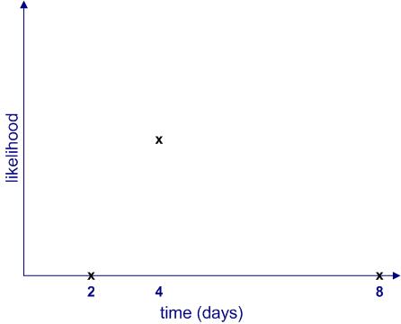
Assume you’ve been asked to do a particular task relating to your area of expertise. From experience you know that this task usually takes 4 days to complete. If things go right, however, it could take as little as 2 days. On the other hand, if things go wrong it could take as long as 8 days. Therefore, your range of possible finish times (outcomes) is anywhere between 2 to 8 days.
Clearly, each of these outcomes is not equally likely. The most likely outcome is that you will finish the task in 4 days. Moreover, the likelihood of finishing in less than 2 days or more than 8 days is zero. If we plot the likelihood of completion against completion time, it would look something like Figure 1.
Figure 1 begs a couple of questions:
- What are the relative likelihoods of completion for all intermediate times – i.e. those between 2 to 4 days and 4 to 8 days?
- How can one quantify the likelihood of intermediate times? In other words, how can one get a numerical value of the likelihood for all times between 2 to 8 days? Note that we know from the earlier discussion that this must be zero for any time less than 2 or greater than 8 days.
The two questions are actually related: as we shall soon see, once we know the relative likelihood of completion at all times (compared to the maximum), we can work out its numerical value.
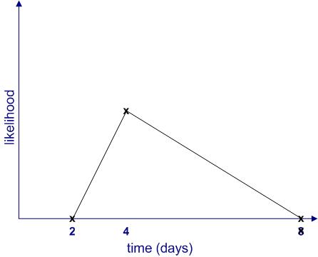
Since we don’t know anything about intermediate times (I’m assuming there is no historical data available, and I’ll have more to say about this later…), the simplest thing to do is to assume that the likelihood increases linearly (as a straight line) from 2 to 4 days and decreases in the same way from 4 to 8 days as shown in Figure 2. This gives us the well-known triangular distribution.
Note: The term distribution is simply a fancy word for a plot of likelihood vs. time.
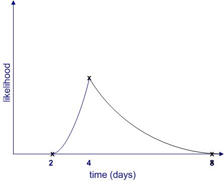
Of course, this isn’t the only possibility; there are an infinite number of others. Figure 3 is another (admittedly weird) example.
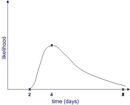
Further, it is quite possible that the upper limit (8 days) is not a hard one. It may be that in exceptional cases the task could take much longer (say, if you call in sick for two weeks) or even not be completed at all (say, if you leave for that mythical greener pasture). Catering for the latter possibility, the shape of the likelihood might resemble Figure 4.
From the figures above, we see that uncertainties are shapes rather than single numbers, a notion popularised by Sam Savage in his book, The Flaw of Averages. Moreover, the “shape of things to come” depends on a host of factors, some of which may not even be on the radar when a future event is being estimated.
Making likelihood precise
Thus far, I have used the word “likelihood” without bothering to define it. It’s time to make the notion more precise. I’ll begin by asking the question: what common sense properties do we expect a quantitative measure of likelihood to have?
Consider the following:
- If an event is impossible, its likelihood should be zero.
- The sum of likelihoods of all possible events should equal complete certainty. That is, it should be a constant. As this constant can be anything, let us define it to be 1.
In terms of the example above, if we denote time by and the likelihood by
then:
for
and
And
where
Where denotes the sum of all non-zero likelihoods – i.e. those that lie between 2 and 8 days. In simple terms this is the area enclosed by the likelihood curves and the x axis in figures 2 to 4. (Technical Note: Since
is a continuous variable, this should be denoted by an integral rather than a simple sum, but this is a technicality that need not concern us here)
is , in fact, what mathematicians call probability– which explains why I have used the symbol
rather than
. Now that I’ve explained what it is, I’ll use the word “probability” instead of ” likelihood” in the remainder of this article.
With these assumptions in hand, we can now obtain numerical values for the probability of completion for all times between 2 and 8 days. This can be figured out by noting that the area under the probability curve (the triangle in figure 2 and the weird shape in figure 3) must equal 1. I won’t go into any further details here, but those interested in the maths for the triangular case may want to take a look at this post where the details have been worked out.
The meaning of it all
(Note: parts of this section borrow from my post on the interpretation of probability in project management)
So now we understand how uncertainty is actually a shape corresponding to a range of possible outcomes, each with their own probability of occurrence. Moreover, we also know, in principle, how the probability can be calculated for any valid value of time (between 2 and 8 days). Nevertheless, we are still left with the question as to what a numerical probability really means.
As a concrete case from the example above, what do we mean when we say that there is 100% chance (probability=1) of finishing within 8 days? Some possible interpretations of such a statement include:
- If the task is done many times over, it will always finish within 8 days. This is called the frequency interpretation of probability, and is the one most commonly described in maths and physics textbooks.
- It is believed that the task will definitely finish within 8 days. This is called the belief interpretation. Note that this interpretation hinges on subjective personal beliefs.
- Based on a comparison to similar tasks, the task will finish within 8 days. This is called the support interpretation.
Note that these interpretations are based on a paper by Glen Shafer. Other papers and textbooks frame these differently.
The first thing to note is how different these interpretations are from each other. For example, the first one offers a seemingly objective interpretation whereas the second one is unabashedly subjective.
So, which is the best – or most correct – one?
A person trained in science or mathematics might claim that the frequency interpretation wins hands down because it lays out an objective, well -defined procedure for calculating probability: simply perform the same task many times and note the completion times.
Problem is, in real life situations it is impossible to carry out exactly the same task over and over again. Sure, it may be possible to do almost the same task, but even straightforward tasks such as vacuuming a room or baking a cake can hold hidden surprise (vacuum cleaners do malfunction and a friend may call when one is mixing the batter for a cake). Moreover, tasks that are complex (as is often the case in the project work) tend to be unique and can never be performed in exactly the same way twice. Consequently, the frequency interpretation is great in theory but not much use in practice.
“That’s OK,” another estimator might say,” when drawing up an estimate, I compared it to other similar tasks that I have done before.”
This is essentially the support interpretation (interpretation 3 above). However, although this seems reasonable, there is a problem: tasks that are superficially similar will differ in the details, and these small differences may turn out to be significant when one is actually carrying out the task. One never knows beforehand which variables are important. For example, my ability to finish a particular task within a stated time depends not only on my skill but also on things such as my workload, stress levels and even my state of mind. There are many external factors that one might not even recognize as being significant. This is a manifestation of the reference class problem.
So where does that leave us? Is probability just a matter of subjective belief?
No, not quite: in reality, estimators will use some or all of three interpretations to arrive at “best guess” probabilities. For example, when estimating a project task, a person will likely use one or more of the following pieces of information:
- Experience with similar tasks.
- Subjective belief regarding task complexity and potential problems. Also, their “gut feeling” of how long they think it ought to take. These factors often drive excess time or padding that people work into their estimates.
- Any relevant historical data (if available)
Clearly, depending on the situation at hand, estimators may be forced to rely on one piece of information more than others. However, when called upon to defend their estimates, estimators may use other arguments to justify their conclusions depending on who they are talking to. For example, in discussions involving managers, they may use hard data presented in a way that supports their estimates, whereas when talking to their peers they may emphasise their gut feeling based on differences between the task at hand and similar ones they have done in the past. Such contradictory representations tend to obscure the means by which the estimates were actually made.
Summing up
Estimates are invariably made in the face of uncertainty. One way to get a handle on this is by estimating the probabilities associated with possible outcomes. Probabilities can be reckoned in a number of different ways. Clearly, when using them in estimation, it is crucial to understand how probabilities have been derived and the assumptions underlying these. We have seen three ways in which probabilities are interpreted corresponding to three different ways in which they are arrived at. In reality, estimators may use a mix of the three approaches so it isn’t always clear how the numerical value should be interpreted. Nevertheless, an awareness of what probability is and its different interpretations may help managers ask the right questions to better understand the estimates made by their teams.
On the accuracy of group estimates
Introduction
The essential idea behind group estimation is that an estimate made by a group is likely to be more accurate than one made by an individual in the group. This notion is the basis for the Delphi method and its variants. In this post, I use arguments involving probabilities to gain some insight into the conditions under which group estimates are more accurate than individual ones.
An insight from conditional probability
Let’s begin with a simple group estimation scenario.
Assume we have two individuals of similar skill who have been asked to provide independent estimates of some quantity, say a project task duration. Further, let us assume that each individual has a probability of making a correct estimate.
Based on the above, the probability that they both make a correct estimate, , is:
,
This is a consequence of our assumption that the individual estimates are independent of each other.
Similarly, the probability that they both get it wrong, , is:
,
Now we can ask the following question:
What is the probability that both individuals make the correct estimate if we know that they have both made the same estimate?
This can be figured out using Bayes’ Theorem, which in the context of the question can be stated as follows:
In the above equation, is the probability that both individuals get it right given that they have made the same estimate (which is what we want to figure out). This is an example of a conditional probability – i.e. the probability that an event occurs given that another, possibly related event has already occurred. See this post for a detailed discussion of conditional probabilities.
Similarly, is the conditional probability that both estimators make the same estimate given that they are both correct. This probability is 1.
Question: Why?
Answer: If both estimators are correct then they must have made the same estimate (i.e. they must both within be an acceptable range of the right answer).
Finally, is the probability that both make the same estimate. This is simply the sum of the probabilities that both get it right and both get it wrong. Expressed in terms of
this is,
.
Now lets apply Bayes’ theorem to the following two cases:
- Both individuals are good estimators – i.e. they have a high probability of making a correct estimate. We’ll assume they both have a 90% chance of getting it right (
).
- Both individuals are poor estimators – i.e. they have a low probability of making a correct estimate. We’ll assume they both have a 30% chance of getting it right (
)
Consider the first case. The probability that both estimators get it right given that they make the same estimate is:
Thus we see that the group estimate has a significantly better chance of being right than the individual ones: a probability of 0.9878 as opposed to 0.9.
In the second case, the probability that both get it right is:
The situation is completely reversed: the group estimate has a much smaller chance of being right than an individual estimate!
In summary: estimates provided by a group consisting of individuals of similar ability working independently are more likely to be right (compared to individual estimates) if the group consists of competent estimators and more likely to be wrong (compared to individual estimates) if the group consists of poor estimators.
Assumptions and complications
I have made a number of simplifying assumptions in the above argument. I discuss these below with some commentary.
- The main assumption is that individuals work independently. This assumption is not valid for many situations. For example, project estimates are often made by a group of people working together. Although one can’t work out what will happen in such situations using the arguments of the previous section, it is reasonable to assume that given the right conditions, estimators will use their collective knowledge to work collaboratively. Other things being equal, such collaboration would lead a group of skilled estimators to reinforce each others’ estimates (which are likely to be quite similar) whereas less skilled ones may spend time arguing over their (possibly different and incorrect) guesses. Based on this, it seems reasonable to conjecture that groups consisting of good estimators will tend to make even better estimates than they would individually whereas those consisting of poor estimators have a significant chance of making worse ones.
- Another assumption is that an estimate is either good or bad. In reality there is a range that is neither good nor bad, but may be acceptable.
- Yet another assumption is that an estimator’s ability can be accurately quantified using a single numerical probability. This is fine providing the number actually represents the person’s estimation ability for the situation at hand. However, typically such probabilities are evaluated on the basis of past estimates. The problem is, every situation is unique and history may not be a good guide to the situation at hand. The best way to address this is to involve people with diverse experience in the estimation exercise. This will almost often lead to a significant spread of estimates which may then have to be refined by debate and negotiation.
Real-life estimation situations have a number of other complications. To begin with, the influence that specific individuals have on the estimation process may vary – a manager who is a poor estimator may, by virtue of his position, have a greater influence than others in a group. This will skew the group estimate by a factor that cannot be estimated. Moreover, strategic behaviour may influence estimates in a myriad other ways. Then there is the groupthink factor as well.
…and I’m sure there are many others.
Finally I should mention that group estimates can depend on the details of the estimation process. For example, research suggests that under certain conditions competition can lead to better estimates than cooperation.
Conclusion
In this post I have attempted to make some general inferences regarding the validity of group estimates based on arguments involving conditional probabilities. The arguments suggest that, all other things being equal, a collective estimate from a bunch of skilled estimators will generally be better than their individual estimates whereas an estimate from a group of less skilled estimators will tend to be worse than their individual estimates. Of course, in real life, there are a host of other factors that can come into play: power, politics and biases being just a few. Though these are often hidden, they can influence group estimates in inestimable ways.
Acknowledgement
Thanks go out to George Gkotsis and Craig Brown for their comments which inspired this post.


