Archive for the ‘Probability’ Category
The drunkard’s dartboard revisited: yet another Excel-based example of Monte Carlo simulation
(Note: An Excel sheet showing sample calculations and plots discussed in this post can be downloaded here.)
Introduction
Some months ago, I wrote a post explaining the basics of Monte Carlo simulation using the example of a drunkard throwing darts at a board. In that post I assumed that the darts could land anywhere on the dartboard with equal probability. In other words, the hit locations were assumed to be uniformly distributed. In a comment on the piece, George Gkotsis challenged this assumption, arguing that that regardless of the level of inebriation of the thrower, a dart would be more likely to land near the centre of the board than away from it (providing the player is at least moderately skilled). He also suggested using the Normal Distribution to model the spread of hits, with the variance of the distribution serving as a rough measure of the inaccuracy (or drunkenness!) of the drunkard. In George’s words:
I would propose to introduce a ‘skill’ factor, which represents the circle/square ratio (maybe a normal-Gaussian distribution). Of course, this skill factor would be very low (high variance) for a drunken player, but would still take into account the fact that throwing darts into a square is not purely random.
In this post I revisit the drunkard’s dartboard, taking into account George’s suggestions.
Setting the stage
To keep things simple, I’ll make the following assumptions:
- The dartboard is a circle of radius 0.5 units centred at the origin (see Figure 1)
- The chance of a hit is greatest at the centre of the dartboard and falls off as one moves away from it.
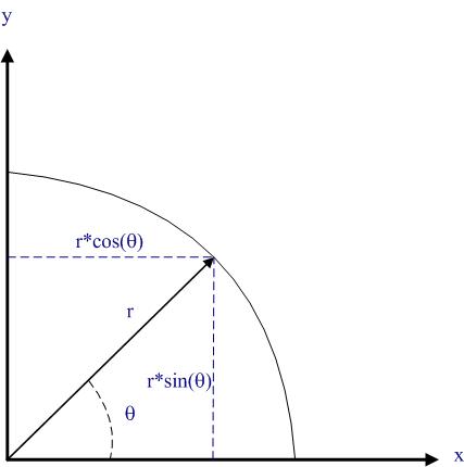
- The distribution of hits is a function of distance from the centre but does not depend on direction. In mathematical terms, for a given distance
from the centre of the dartboard, the dart can land at any angle
with equal probability,
being the angle between the line joining the centre of the board to the dart and the x axis. See Figure 2 for graphical representations of a hit location in terms of
and
. Note that that the
and
coordinates can be obtained using the formulas
and
as s shown in Figure 2.
- Hits are distributed according to the Normal distribution with maximum at the centre of the dartboard.
- The variance of the Normal distribution is a measure of inaccuracy/drunkenness of the drunkard: the more drunk the drunk, the greater the variation in his aim.
These assumptions are consistent with George’s suggestions.
The simulation
[Note to the reader: you may want to download the demo before continuing.]
The steps of a simulation run are as follows:
- Generate a number that is normally distributed with a zero mean and a specified standard deviation. This gives the distance,
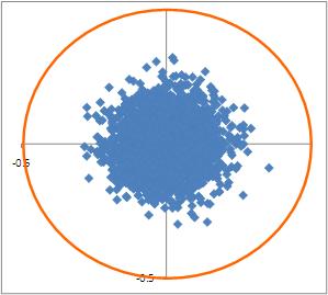
, of a randomly thrown dart from the centre of the board for a player with a “inaccuracy factor” represented by the standard deviation. Column A in the demo contains normally distributed random numbers with zero mean and a standard deviation of 0.2 . Note that I selected the latter number for no other reason than the results show up clearly on a fixed-axis plot shown in Figure 2.
- Generate a uniformly distributed random number lying between 0 and
. This represents the angle
. This is the content of column B of the demo.
- The numbers obtained from steps 1 and 2 for completely specify the location of a hit. The location’s
and
coordinates can be worked out using the formulas
and
. These are listed in columns C and D in the Excel demo.
- Re-run steps 1 through 4 as many times as needed. Note that the demo is set up for 5000 runs. You can change this manually or, better yet, automate it. The latter is left as an exercise for you.
It is instructive to visualize the resulting hits using a scatter plot. Among other things this can tell you, at a glance, if the results make sense. For example, we would expect hits to be symmetrically distributed about the origin because the drunkard’s throws are not biased in any particular direction around the centre). A non-symmetrical distribution is thus an indication that there is an error in the calculations.
Now, any finite collection of hits is unlikely to be perfectly symmetrical because of outliers. Nevertheless, the distributions should be symmetrical on average. To test this, run the demo a few times (hit F9 with the demo open). Notice how the position of outliers and the overall shape of the distribution of points changes randomly from simulation to simulation. In all cases, however, there is a clear maximum at the centre of the dartboard with the probability of a hit falling with distance from the centre.
Figure 3 shows the results of simulations for a standard deviation of 0.2. Figures 4 and 5 show the results of simulations for standard deviations of 0.1 and 0.4.
Note that the plot has fixed axes- i.e. the area depicted is the 1×1 square that encloses the dartboard, regardless of the standard deviation. Consequently, for larger standard deviations (such as 0.4) many hits will be out of range and will not show up on the plot.
Closing remarks
As I have stressed in my previous posts on Monte Carlo simulation, the usefulness of a simulation depends on the choice of an appropriate distribution. If the selected distribution does not reflect reality, neither will the simulation. This is true regardless of whether one is simulating a drunkard’s wayward aim or the duration of project task. You may have noted that the assumption of normally-distributed hits has no justification whatsoever; it is just as arbitrary as my original assumption of uniformity. In fact, the hit locations of drunken dart throws is highly unlikely to be either uniform or Normal. Nevertheless, I hope that some of my readers will find the above example to be of pedagogical value.
Acknowledgement
Thanks to George Gkotsis for his comment which got me thinking about this post.
Uncertainty about uncertainty
Introduction
More often than not, managerial decisions are made on the basis of uncertain information. To lend some rigour to the process of decision making, it is sometimes assumed that uncertainties of interest can be quantified accurately using probabilities. As it turns out, this assumption can be incorrect in many situations because the probabilities themselves can be uncertain. In this post I discuss a couple of ways in which such uncertainty about uncertainty can manifest itself.
The problem of vagueness
In a paper entitled, “Is Probability the Only Coherent Approach to Uncertainty?”, Mark Colyvan made a distinction between two types of uncertainty:
- Uncertainty about some underlying fact. For example, we might be uncertain about the cost of a project – that there will be a cost is a fact, but we are uncertain about what exactly it will be.
- Uncertainty about situations where there is no underlying fact. For example, we might be uncertain about whether customers will be satisfied with the outcome of a project. The problem here is the definition of customer satisfaction. How do we measure it? What about customers who are neither satisfied nor dissatisfied? There is no clear-cut definition of what customer satisfaction actually is.
The first type of uncertainty refers to the lack of knowledge about something that we know exists. This is sometimes referred to as epistemic uncertainty – i.e. uncertainty pertaining to knowledge. Such uncertainty arises from imprecise measurements, changes in the object of interest etc. The key point is that we know for certain that the item of interest has well-defined properties, but we don’t know what they are and hence the uncertainty. Such uncertainty can be quantified accurately using probability.
Vagueness, on the other hand, arises from an imprecise use of language. Specifically, the term refers to the use of criteria that cannot distinguish between borderline cases. Let’s clarify this using the example discussed earlier. A popular way to measure customer satisfaction is through surveys. Such surveys may be able to tell us that customer A is more satisfied than customer B. However, they cannot distinguish between borderline cases because any boundary between satisfied and not satisfied customers is arbitrary. This problem becomes apparent when considering an indifferent customer. How should such a customer be classified – satisfied or not satisfied? Further, what about customers who choose not to respond? It is therefore clear that any numerical probability computed from such data cannot be considered accurate. In other words, the probability itself is uncertain.
Ambiguity in classification
Although the distinction made by Colyvan is important, there is a deeper issue that can afflict uncertainties that appear to be quantifiable at first sight. To understand how this happens, we’ll first need to take a brief look at how probabilities are usually computed.
An operational definition of probability is that it is the ratio of the number of times the event of interest occurs to the total number of events observed. For example, if my manager notes my arrival times at work over 100 days and finds that I arrive before 8:00 am on 62 days then he could infer that the probability my arriving before 8:00 am is 0.62. Since the probability is assumed to equal the frequency of occurrence of the event of interest, this is sometimes called the frequentist interpretation of probability.
The above seems straightforward enough, so you might be asking: where’s the problem?
The problem is that events can generally be classified in several different ways and the computed probability of an event occurring can depend on the way that it is classified. This is called the reference class problem. In a paper entitled, “The Reference Class Problem is Your Problem Too”, Alan Hajek described the reference class problem as follows:
“The reference class problem arises when we want to assign a probability to a proposition (or sentence, or event) X, which may be classified in various ways, yet its probability can change depending on how it is classified.”
Consider the situation I mentioned earlier. My manager’s approach seems reasonable, but there is a problem with it: all days are not the same as far as my arrival times are concerned. For example, it is quite possible that my arrival time is affected by the weather: I may arrive later on rainy days than on sunny ones. So, to get a better estimate my manager should also factor in the weather. He would then end up with two probabilities, one for fine weather and the other for foul. However, that is not all: there are a number of other criteria that could affect my arrival times – for example, my state of health (I may call in sick and not come in to work at all), whether I worked late the previous day etc.
What seemed like a straightforward problem is no longer so because of the uncertainty regarding which reference class is the right one to use.
Before closing this section, I should mention that the reference class problem has implications for many professional disciplines. I have discussed its relevance to project management in my post entitled, “The reference class problem and its implications for project management”.
To conclude
In this post we have looked at a couple of forms of uncertainty about uncertainty that have practical implications for decision makers. In particular, we have seen that probabilities used in managerial decision making can be uncertain because of vague definitions of events and/or ambiguities in their classification. The bottom line for those who use probabilities to support decision-making is to ensure that the criteria used to determine events of interest refer to unambiguous facts that are appropriate to the situation at hand. To sum up: decisions made on the basis of probabilities are only as good as the assumptions that go into them, and the assumptions themselves may be prone to uncertainties such as the ones described in this article.
The drunkard’s dartboard: an intuitive explanation of Monte Carlo methods
(Note to the reader: An Excel sheet showing sample calculations and plots discussed in this post can be downloaded here.)
Monte Carlo simulation techniques have been applied to areas ranging from physics to project management. In earlier posts, I discussed how these methods can be used to simulate project task durations (see this post and this one for example). In those articles, I described simulation procedures in enough detail for readers to be able to reproduce the calculations for themselves. However, as my friend Paul Culmsee mentioned, the mathematics tends to obscure the rationale behind the technique. Indeed, at first sight it seems somewhat paradoxical that one can get accurate answers via random numbers. In this post, I illustrate the basic idea behind Monte Carlo methods through an example that involves nothing more complicated than squares and circles. To begin with, however, I’ll start with something even simpler – a drunken darts player.
Consider a sozzled soul who is throwing darts at a board situated some distance from him. To keep things simple, we’ll assume the following:
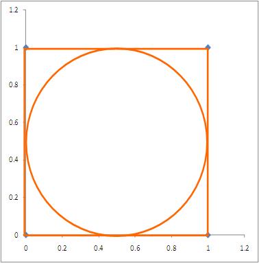
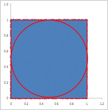
- The board is modeled by the circle shown in Figure 1, and our souse scores a point if the dart falls within the circle.
- The dart board is inscribed in a square with sides 1 unit long as shown in the figure, and we’ll assume for simplicity that the dart always falls somewhere within the square (our protagonist is not that smashed).
- Given his state, our hero’s aim is not quite what it should be – his darts fall anywhere within the square with equal probability. (Note added on 01 March 2011: See the comment by George Gkotsis below for a critique of this assumption)
We can simulate the results of our protagonist’s unsteady attempts by generating two sets of uniformly distributed random numbers lying between 0 and 1 (This is easily done in Excel using the rand() function). The pairs of random numbers thus generated – one from each set – can be treated as the (x,y) coordinates of the dart for a particular throw. The result of 1000 pairs of random numbers thus generated (representing the drunkard’s dart throwing attempts) is shown in Figure 2 (For those interested in seeing the details, an Excel sheet showing the calculations for 100o trials can be downloaded here).
A trial results in a “hit” if it lies within the circle. That is, if it satisfies the following equation:
(Note: if we replace “<” by “=” in the above expression, we get the equation for a circle of radius 0.5 units, centered at x=0.5 and y=0.5.)
Now, according to the frequency interpretation of probability, the probability of the plastered player scoring a point is approximated by the ratio of the number of hits in the circle to the total number of attempts. In this case, I get an average of 790/1000 which is 0.79 (generated from 10 sets of 1000 trials each). Your result will be different from because you will generate different sets of random numbers from the ones I did. However, it should be reasonably close to my result.
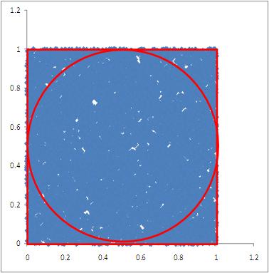
Further, the frequency interpretation of probability tells us that the approximation becomes more accurate as the number of trials increases. To see why this is so, let’s increase the number of trials and plot the results. I carried out simulations for 2000, 4000, 8000 and 16000 trials. The results of these simulations are shown in Figures 3 through 6.
Since a dart is equally likely to end up anywhere within the square, the exact probability of a hit is simply the area of the dartboard (i.e. the circle) divided by the entire area over which the dart can land. In this case, since the area of the enclosure (where the dart must fall) is 1 square unit, the area of the dartboard is actually equal to the probability. This is easily seen by calculating the area of the circle using the standard formula where
is the radius of the circle (0.5 units in this case). This yields 0.785398 sq units, which is reasonably close to the number that we got for the 1000 trial case. In the 16000 trial case, I get a number that’s closer to the exact result: an average of 0.7860 from 10 sets of 16000 trials.
As we see from Figure 6, in the 16000 trial case, the entire square is peppered with closely-spaced “dart marks” – so much so, that it looks as though the square is a uniform blue. Hence, it seems intuitively clear that as we increase, the number of throws, we should get a better approximation of the area and, hence, the probability.
There are a couple of points worth mentioning here. First, in principle this technique can be used to calculate areas of figures of any shape. However, the more irregular the figure, the worse the approximation – simply because it becomes less likely that the entire figure will be sampled correctly by “dart throws.” Second, the reader may have noted that although the 16000 trial case gives a good enough result for the area of the circle, it isn’t particularly accurate considering the large number of trials. Indeed, it is known that the “dart approximation” is not a very good way of calculating areas – see this note for more on this point.
Finally, let’s look at connection between the general approach used in Monte Carlo techniques and the example discussed above (I use the steps described in the Wikipedia article on Monte Carlo methods as representative of the general approach):
- Define a domain of possible inputs – in our case the domain of inputs is defined by the enclosing square of side 1 unit.
- Generate inputs randomly from the domain using a certain specified probability distribution – in our example the probability distribution is a pair of independent, uniformly distributed random numbers lying between 0 and 1.
- Perform a computation using the inputs – this is the calculation that determines whether or not a particular trial is a hit or not (i.e. if the x,y coordinates obey inequality (1) it is a hit, else it’s a miss)
- Aggregate the results of the individual computations into the final result – This corresponds to the calculation of the probability (or equivalently, the area of the circle) by aggregating the number of hits for each set of trials.
To summarise: Monte Carlo algorithms generate random variables (such as probability) according to pre-specified distributions. In most practical applications one will use more efficient techniques to sample the distribution (rather than the naïve method I’ve used here.) However, the basic idea is as simple as playing drunkard’s darts.
Acknowledgements
Thanks go out to Vlado Bokan for helpful conversations while this post was being written and to Paul Culmsee for getting me thinking about a simple way to explain Monte Carlo methods.

