Probability | Eight to Late

Archive for the ‘Probability’ Category

Trumped by conditionality: why many posts on this blog are not interesting

Introduction

A large number of the posts on this blog do not get much attention – not too many hits and few if any comments. There could be several reasons for this, but I need to consider the possibility that readers find many of the things I write about uninteresting. Now, this isn’t for the want of effort from my side: I put a fair bit of work into research and writing, so it is a little disappointing. However, I take heart from the possibility that it might not be entirely my fault: there’s a statistical reason (excuse?) for the dearth of quality posts on this blog. This (possibly uninteresting) post discusses this probabilistic excuse.

The argument I present uses the concepts of conditional probability and Bayes Theorem. Those unfamiliar with these may want to have a look at my post on Bayes theorem before proceeding further.

The argument

Grist for my blogging mill comes from a variety of sources: work, others’ stories, books, research papers and the Internet. Because of time constraints, I can write up only a fraction of the ideas that come to my attention. Let’s put a number to this fraction – say I can write up only 10% of the ideas I come across. Assuming that my intent is to write interesting stuff, this number corresponds to the best (or most interesting) ideas I encounter. Of course, the term “interesting” is subjective – an idea that fascinates me might not have the same effect on you. However this is a problem for most qualitative judgements, so we’ll accept this and move on.

If we denote the event “I have an interesting idea” by $I$ and its probability by $P(I)$ , we have:

$P(I) = 0.1$

Then, if we denote the event “I have an idea that is uninteresting” by $U$ , we have:

$P(U) = 0.9$ ,

assuming that an idea must either be interesting or uninteresting (no other possibilities allowed).

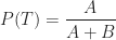
Now, for me to write up an idea, I have to find it interesting (i.e. judge it as being in the top 10%). Let’s be generous and assume that I correctly recognise an interesting idea (as being interesting) 70% of the time. From this, the conditional probability of my writing a post given that I encounter an interesting idea, $P(W|I)$ , is:

$P(W|I) = 0.7$ ,

where $W$ is the event that I write up an idea.

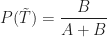
On the flip side, let’s assume that I correctly recognise 80% of the uninteresting ideas that I encounter as being no good. This implies that I incorrectly identify 20% of the uninteresting stuff as being interesting. That is, 20% of the uninteresting stuff is wrongly identified as being blog-worthy. So, the conditional probability of my writing a post about an uninteresting idea, $P(W|U)$ , is:

$P(W|U) = 0.2$

(If the above values for $P(W|I)$ and $P(W|U)$ are confusing remember that, by assumption, I write about all ideas that I find interesting – and this includes those ideas that I deem interesting but are actually uninteresting)

Now, we want to figure out the probability that a post that appears on my blog is interesting – i.e. that a post is interesting given that I have written it up. Using the notation of conditional probability, this can be written as $P(I|W)$ . Bayes Theorem tells us that:

$P(I|W) = \displaystyle\frac{P(W|I) * P(I)}{P(W)}$

$P(W)$ , which is the probability that I write a post, can be expressed as follows:

$P(W)$ = probability that I write an interesting post+ probability that I write an uninteresting post

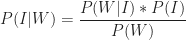
This can be written as,

$P(W) = P(W|I) * P(I) + P(W|U) * P(U)$

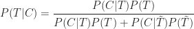
Substituting this in the expression for Bayes Theorem, we get:

$P(I|W) = \displaystyle \frac{P(W|I) * P(I)}{P(W|I) * P(I) + P(W|U) * P(U)}$

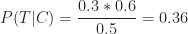
Using the numbers quoted above

$P(I|W) =\displaystyle \frac{0.7*0.1}{0.7*0.1+0.2*0.9}=0.28$

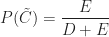
So, only 28% of the ideas I write about are interesting. The main reason for is my inability to filter out all the dross. These “false positives” – which are all the ideas that I identify as interesting but are actually not – are represented by the $P(W|U) * P(U)$ term in the denominator. Since there are way more bad ideas than good ones floating around (pretty much everywhere!), the chance of false positives is significant.

So, there you go: it isn’t my fault really. 🙂

I should point out that the percentage of interesting ideas written up will be small whenever the false positive term is significant compared to the numerator. In this sense the result is insensitive to the values of the probabilities that I’ve used.

Of course, the argument presented above is based on a number of assumptions. I assume that:

Mostreaders of this blog share my interests.
The ideas that I encounter are either interesting or uninteresting.
There is an arbitrary cutoff point between interesting and uninteresting ideas (the 10% cutoff).
There is an objective criterion for what’s interesting and what’s not, and that I can tell one from the other 70% of the time.
The relevant probabilities are known.

…and so, to conclude

I have to accept that much of the stuff I write about will be uninteresting, but can take consolation in the possibility that it is a consequence of conditional probabilities. I’m trumped by conditionality, once more.

Acknowledgements

This post was inspired by Peter Rousseeuw’s brilliant and entertaining paper entitled, Why the Wrong Papers Get Published. Thanks also go out to Vlado Bokan for interesting conversations about conditional probabilities and Bayes theorem.

Written by K

March 17, 2010 at 10:43 pm

Posted in Bias, Estimation, Probability, Statistics

Bayes Theorem for project managers

with 10 comments

Introduction

Projects are fraught with uncertainty, so it is no surprise that the language and tools of probability are making their way into project management practice. A good example of this is the use of Monte Carlo methods to estimate project variables. Such tools enable the project manager to present estimates in terms of probabilities (e.g. there’s a 90% chance that a project will finish on time) rather than illusory certainties. Now, it often happens that we want to find the probability of an event occurring given that another event has occurred. For example, one might want to find the probability that a project will finish on time given that a major scope change has already occurred. Such conditional probabilities, as they are referred to in statistics, can be evaluated using Bayes Theorem. This post is a discussion of Bayes Theorem using an example from project management.

Bayes theorem by example

All project managers want to know whether the projects they’re working on will finish on time. So, as our example, we’ll assume that a project manager asks the question: what’s the probability that my project will finish on time? There are only two possibilties here: either the project finishes on (or before) time or it doesn’t. Let’s express this formally. Denoting the event the project finishes on (or before) time by $T$ , the event the project does not finish on (or before) time by $\tilde T$ and the probabilities of the two by $P(T)$ and $P(\tilde T)$ respectively, we have:

$P(T)+P(\tilde T) = 1$ ……(1),

Equation (1) is simply a statement of the fact that the sum of the probabilities of all possible outcomes must equal 1.

Fig 1. is a pictorial representation of the two events and how they relate to the entire universe of projects done by the organisation our project manager works in. The rectangular areas $A$ and $B$ represent the on time and not on time projects, and the sum of the two areas, $A+B$ , represents all projects that have been carried out by the organisation.

Fig 1: On Time and Not on Time projects

In terms of areas, the probabilities quoted above can be expressed as:

$P(T) = \displaystyle \frac{A}{A+B}$ ……(2),

and

$P(\tilde T) = \displaystyle \frac{B}{A+B}$ ……(3).

This also makes explicit the fact that the sum of the two probabilities must add up to one.

Now, there are several variables that can affect project completion time. Let’s look at just one of them: scope change. Let’s denote the event “there is a major change of scope” by $C$ and the complementary event (that there is no major change of scope) by $\tilde C$ .

Again, since the two possibilities cover the entire spectrum of outcomes, we have:

$P(C)+P(\tilde C) = 1$ ……(4).

Fig 2. is a pictorial representation of by $C$ and $\tilde C$ .

Fig 2: "Major Change" and "No Major Change" projects

The rectangular areas $D$ and $E$ represent the projects that have undergone major scope changes and those that haven’t respectively.

$P(C) = \displaystyle \frac{D}{D+E}$ ……(5),

and

$P(\tilde C) = \displaystyle \frac{E}{D+E}$ ……(6).

Clearly we also have 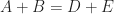$A+B=D+E$ since the number of projects completed is a fixed number, regardless of how it is arrived at.

Now things get interesting. One could ask the question: What is the probability of finishing on time given that there has been a major scope change? This is a conditional probability because it represents the likelihood that something will happen (on-time completion) on the condition that something else has already happened (scope change).

As a first step to answering the question posed in the previous paragraph, let’s combine the two events graphically. Fig 3 is a combination of Figs 1 and 2. It shows four possible events:

On Time with Major Change ( $T$ , $C$ ) – denoted by the rectangular area $AD$ in Fig 3.
On Time with No Major Change ( $T$ , $\tilde C$ ) – denoted by the rectangular area $AE$ in Fig 3.
Not On Time with Major Change ( $\tilde T$ , $C$ ) – denoted by the rectangular area $BD$ in Fig 3.
Not On Time with No Major Change ( $\tilde T$ , $\tilde latex C$) – denoted by the rectangular area $BE$ in Fig 3.

Fig 3: Combination of events shown in Figs 1 and 2

We’re interested in the probability that the project finishes on time given that it has suffered a major change in scope. In the notation of conditional probability, this is denoted by $P(T|C)$ . In terms of areas, this can be expressed as

$P(T|C) = \displaystyle \frac{AD}{AD+BD} = \frac{AD}{D}$ ……(7) ,

since $D$ (or equivalently $AD+BD$ ) represent all projects that have undergone a major scope change.

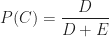
Similarly, the conditional probability that a project has undergone a major change given that it has come in on time, $P(C|T)$ , can be written as:

$P(C|T) =\displaystyle \frac{AD}{AD+AE} = \frac{AD}{A}$ ……(8) ,

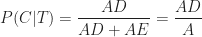
since $AD+AE=A$ .

Now, what I’m about to do next may seem like pointless algebraic jugglery, but bear with me…

Consider the ratio of the area $AD$ to the big outer rectangle (whose area is $A+B$ ) . This ratio can be expressed as follows:

$\displaystyle\frac{AD}{A+B}=\frac{AD}{D}\times\frac{D}{A+B}=\frac{AD}{A}\times\frac{A}{A+B}$ ……(9).

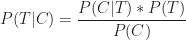
This is simply multiplying and dividing by the same factor ( $D$ in the second expression and $A$ in the third.

Written in the notation of conditional probabilities, the second and third expressions in (9) are:

$P(T|C)*P(C)=P(C|T)*P(T)$ ……(10),

which is Bayes theorem.

From the above discussion, it should be clear that Bayes theorem follows from the definition of conditional probability.

We can rewrite Bayes theorem in several equivalent ways:

$P(T|C)=\displaystyle\frac{P(C|T)*P(T)}{P(C)}$ ……(11),

$P(T|C)=\displaystyle\frac{P(C|T)P(T)}{ P(C|T)P(T)+P(C|\tilde T)P(\tilde T)}$ ……(12),

where the denominator in (12) follows from the fact that a project that undergoes a major change will either be on time or will not be on time (there is no other possibility).

A numerical example

To complete the discussion, let’s look at a numerical example.

Assume our project manager has historical data on projects that have been carried out within the organisation. On analyzing the data, the PM finds that 60% of all projects finished on time. This implies:

$P(T) = 0.6$ ……(13),

and

$P(T) = 0.4$ ……(13),

Let us assume that our organisation also tracks major changes made to projects in progress. Say 50% of all historical projects are found to have major changes. This implies:

$P(C) = 0.5$ ……(15).

Finally, let us assume that our project manager has access to detailed data on successful projects, and that an analysis of this data shows that 30% on time projects have undergone at least one major scope change. This gives:

$P(C|T) = 0.3$ ……(16).

Equations (13) through (16) give us the numbers we need to calculated $P(T|C)$ using Bayes Theorem. Plugging the numbers in equation (11), we get:

$P(T|C)=\displaystyle\frac{0.3*0.6}{0.5}=0 .36$ ……(16)

So, in this organisation, if a project undergoes a major change then there’s a 36% probability that it will finish on time. Compare this to the 60% (unconditional) probability of finishing on time. Bayes theorem enables the project manager to quantify the impact of change in scope on project completion time, providing the relevant historical data is available. The italicised bit in the previous sentence is important; I’ll have more to say about it in the concluding section.

In closing this section I should emphasise that although my discussion of Bayes theorem is couched in terms of project completion times and scope changes, the arguments used are general. Bayes theorem holds for any pair of events.

Concluding remarks

It should be clear that the probability calculated in the previous section is an extrapolation based on past experience. In this sense, Bayes Theorem is a formal statement of the belief that one can predict the future based on past events. This goes beyond probability theory; it is an assumption that underlies much of science. It is important to emphasise that the prediction is based on enumeration, not analysis: it is solely based on ratios of the number of projects in one category versus the other; there is no attempt at finding a causal connection between the events of interest. In other words, Bayes theorem suggests there is a correlation between major changes in scope and delays, but it does not tell us why. The latter question can be answered only via a detailed study which might culminate in a theory that explains the causal connection between changes in scope and completion times.

It is also important to emphasise that data used in calculations should be based on events that akin to the one at hand. In the case of the example, I have assumed that historical data is for projects that resemble the one the project manager is working on. This assumption must be validated because there could be situations in which a major change in scope actually reduces completion time (when the project is “scoped-down”, for instance). In such cases, one would need to ensure that the numbers that go into Bayes theorem are based on historical data for “scoped-down” projects only.

To sum up: Bayes theorem expresses a fundamental relationship between conditional probabilities of two events. Its main utility is that it enables us to make probabilistic predictions based on past events; something that a project manager needs to do quite often. In this post I’ve attempted to provide a straightforward explanation of Bayes theorem – how it comes about and what its good for. I hope I’ve succeeded in doing so. But if you’ve found my explanation confusing, I can do no better than to direct you to a couple of excellent references.

Communicating risks using the Improbability Scale

with 3 comments

It can be hard to develop an intutitive feel for a probability that is expressed in terms of a single number. The main reason for this is that a numerical probability, without anything to compare it to, may not convey a sense of how likely (or unlikely) an event is. For example, the NSW Road Transport Authority tells us that 0.97% of the registered vehicles on the road in NSW in 2008 were involved in at least one accident. Based on this, the probability that a randomly chosen vehicle will be involved in an accident over a period of one year is 0.0097. Although this number suggests the risk is small, it begs the question: how small? How does it compare to the probability of other, known events? In a short paper entitled, The Improbability Scale, David Ritchie outlines how to make this comparison in an inituitively appealing way.

Ritchie defines the Improbability Scale, $I$ , as:

$I = - \log (p)$

where $p$ is the probability of the event.

By definition, $I$ is 0 for absolutely certain events ( $p=1$ ), and increases as $p$ decreases. The advantage of using $I$ (as opposed to $p$ ) is that, in most case, $I$ , will be a number between 0 and 10. An $I$ of 10 corresponds to a probability of 0.0000000001, which is so small that the event it refers to is practically impossible.

Let’s look at the improbability of some events expressed in terms of $I$ .

Rolling a six on the throw of a die. $p$ = 1/6; $I$ = 0.8.
Picking a specific card (say the 10 of diamonds) from a pack (wildcards excluded). $p$ = 1/52; $I$ = 1.7.
A (particular) vehicle being involved in at least one accident in the Australian state of NSW over a period of one year (the example quoted in the in the first paragraph). $p$ = .0097; $I$ = 2.0.
One’s birthday occurring on a randomly picked day of the year. $p$ = 1/365; $I$ = 2.6.
Probability of getting 10 heads in 10 consecutive coin tosses. $p$ = $(0.5)^{10}$ (or 0.00098 ); $I$ = 3
Drawing 5 sequential cards of the same suit from a complete deck (a straight flush). $p$ = 0.0000139; $I$ = 4.9 (Note: This can be calculated by dividing the total number of sequential 5 card hands and dividing it by the total number of 5 card hands from a deck of 52. I’m too lazy to do the calculation myself, but it’s explained in this Wikipedia article if you’re interested. )
Being struck by lightning in Australia. $p$ = 1/1600000; $I$ = 6.2. (source: this article from Australian Geographic – the article doesn’t say over what period, but I reckon it’s per year)
Winning the Oz Lotto Jackpot. $p$ = $2.204 \times 10^{-8}$ ; $I$ = 7.7 (based on odds from NSW lotteries for a single game)

Apart from clarifying the risk of a traffic accident, this tells me (quite unambiguously!) that I must stop buying lottery tickets.

A side benefit of the improbability scale is that it eases the tasks of calculating the probability of combined events. If two events are independent, the probability that they will occur together is given by the product of their individual probabilities of occurrence. Since the logarithm of a product of two number equals the sum of the numbers, $I$ for the combined event is obtained by adding their individual $I$ values. So the $I$ for throwing a six and drawing a specific card from a deck is 2.5 (that is, 0.8+1.7), making it more unlikely than being involved in a vehicle accident. That certainly puts both probabilities in perspective.

In short: the improbability scale offers a nice way to understand the likelihood of an event occuring in comparison to other events. In particular, the examples discussed above show how it can be used to illustrate and communicate the likelihood of risks in a vivid and intuitive manner.

Written by K

February 23, 2010 at 10:15 pm

Posted in Communication, Paper Review, Probability, Risk analysis, Statistics

Eight to Late

Archive for the ‘Probability’ Category

Trumped by conditionality: why many posts on this blog are not interesting

Introduction

The argument

…and so, to conclude

Bayes Theorem for project managers

Introduction

Bayes theorem by example

A numerical example

Concluding remarks

Recommended Reading

Communicating risks using the Improbability Scale

Subscribe

Search

Author

Copyright

My book

Top Posts & Pages

Recent Posts

Categories

Archives

Blogroll

Other links

Eight to Late

Archive for the ‘Probability’ Category

Trumped by conditionality: why many posts on this blog are not interesting

Introduction

The argument

…and so, to conclude

Rate this:

Share this:

Bayes Theorem for project managers

Introduction

Bayes theorem by example

A numerical example

Concluding remarks

Recommended Reading

Rate this:

Share this:

Communicating risks using the Improbability Scale

Rate this:

Share this:

Subscribe

Search

Author

Copyright

My book

Top Posts & Pages

Recent Posts

Categories

Archives

Blogroll

Other links