Archive for the ‘Statistics’ Category
Monte Carlo simulation of risk and uncertainty in project tasks
Introduction
When developing duration estimates for a project task, it is useful to make a distinction between the uncertainty inherent in the task and uncertainty due to known risks. The former is uncertainty due to factors that are not known whereas the latter corresponds uncertainty due to events that are known, but may or may not occur. In this post, I illustrate how the two types of uncertainty can be combined via Monte Carlo simulation. Readers may find it helpful to keep my introduction to Monte Carlo simulations of project tasks handy, as I refer to it extensively in the present piece.
Setting the stage
Let’s assume that there’s a task that needs doing, and the person who is going to do it reckons it will take between 2 and 8 hours to complete it, with a most likely completion time of 4 hours. How the estimator comes up with these numbers isn’t important here – maybe there’s some guesswork, maybe some padding or maybe it is really based on experience (as it should be). For simplicity we’ll assume the probability distribution for the task duration is triangular. It is not hard to show that, given the above mentioned estimates, the probability, 

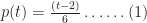

And,
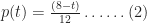
These two expressions are sometimes referred to as the probability distribution function (PDF). The PDF described by equations (1) and (2) is illustrated in Figure 1. (Note: Please click on the Figures to view full-size images)

Figure 1: Probability distribution for task
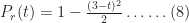
Now, a PDF tells us the probability that the task will finish at a particular time 


and,

For a detailed derivation, please see my introductory post. The CDF for the distribution is shown in Figure 2.

Figure 2: CDF for task
Now for the complicating factor: let us assume there is a risk that has a bearing on this task. The risk could be any known factor that has a negative impact on task duration. For example, it could be that a required resource is delayed or that the deliverable will fails a quality check and needs rework. The consequence of the risk – should it eventuate – is that the task takes longer. How much longer the task takes depends on specifics of the risk. For the purpose of this example we’ll assume that the additional time taken is also described by a triangular distribution with a minimum, most likely and maximum time of 1, 2 and 3 hrs respectively. The PDF 

And

The figure for this distribution is shown in Figure 3.

Figure 3: Probability distribution of additional time due to risk
The CDF for the additional time taken if the risk eventuates (which we’ll denote by 

and,
The CDF for the risk consequence is shown in Figure 4.

Figure 4: CDF of additional time due to risk
Before proceeding with the simulation it is worth clarifying what all this means, and what we want to do with it.
Firstly, equations 1-4 describe the inherent uncertainty associated with the task while equations 5 through 8 describe the consequences of the risk, if it eventuates.
Secondly, we have described the task and the risk separately. In reality, we need a unified description of the two – a combined distribution function for the uncertainty associated with the task and the risk taken together. This is what the simulation will give us.
Finally, one thing I have not yet specified is the probabilty that the risk will actually occur. Clearly, the higher the probability, the greater the potential delay. Below I carry out simulations for risk probabilities of varying from 0.1 to 0.5.
That completes the specification of the problem – let’s move on to the simulation.
The simulation
The simulation procedure I used for the zero-risk case (i.e. the task described by equations 1 and 2 ) is as follows :
- Generate a random number between 0 and 1. Treat this number as the cumulative probability,
- Find the time,
- Repeat steps (1) and (2) for a sufficiently large number of trials.
The frequency distribution of completion times for the task, based on 30,000 trials is shown in Figure 5.

Figure 5: Simulation histogram for zero-risk case
As we might expect, Figure 5 can be translated to the probability distribution shown in Figure 1 by a straightforward normalization – i.e. by dividing each bar by the total number of trials.
What remains to be done is to incorporate the risk (as modeled in equations 5-6) into the simulation. To simulate the task with the risk, we simply do the following for each trial:
- Simulate the task without the risk as described earlier.
- Generate another random number between 0 and 1.
- If the random number is less than the probability of the risk, then simulate the risk. Note that since the risk is described by a triangular function, the procedure to simulate it is the same as that for the task (albeit with different parameters).
- If the random number is greater than the probability of the risk, do nothing.
- Add the results of 1 and 4. This is the outcome of the trial.
- Repeat steps 1-5 for as many trials as required.
I performed simulations for the task with risk probabilities of 10%, 30% and 50%. The frequency distributions of completion times for these are displayed in Figures 6-8 (in increasing order of probability). As one would expect, the spread of times increases with increasing probability. Further, the distribution takes on a distinct second peak as the probability increases: the first peak is at 


Figure 6: Simulation histogram (10% probability of risk)

Figure 7: Simulation histogram (30% probability of risk)

Figure 8: Frequency histogram (50% probability of risk)
It is also instructive to compare average completion times for the four cases (zero-risk and 10%, 30% and 50%). The average can computed from the simulation by simply adding up the simulated completion times (for all trials) and dividing by the total number of simulation trials (30,000 in our case). On doing this, I get the following:
Average completion time for zero-risk case = 4.66 hr
Average completion time with 10% probability of risk = 4.89 hrs
Average completion time with 30% probability of risk = 5.36 hrs
Average completion time with 50% probability of risk= 5.83 hrs
No surprises here.
One point to note is that the result obtained from the simulation for the zero-risk case compares well with the exact formula for a triangular distribution (see the Wikipedia article for the triangular distribution):

This serves as a sanity check on the simulation procedure.
It is also interesting to compare the cumulative probabilities of completion in the zero-risk and high risk (50% probability) case. The CDFs for the two are shown in Figure 9. The co-plotted CDFs allow for a quick comparison of completion time predictions. For example, in the zero-risk case, there is about a 90% chance that the task will be completed in a little over 6 hrs whereas when the probability of the risk is 50%, the 90% completion time increases to 8 hrs (see Figure 9).

Figure 9: CDFs for zero risk and 50% probability of risk cases
Next steps and wrap up
For those who want to learn more about simulating project uncertainty and risk, I can recommend the UK MOD paper – Three Point Estimates And Quantitative Risk Analysis A Process Guide For Risk Practitioners. The paper provides useful advice on how three point estimates for project variables should be constructed. It also has a good discussion of risk and how it should be combined with the inherent uncertainty associated with a variable. Indeed, the example I have described above was inspired by the paper’s discussion of uncertainty and risk.
Of course, as with any quantitative predictions of project variables, the numbers are only as reliable as the assumptions that go into them, the main assumption here being the three point estimates that were used to derive the distributions for the task uncertainty and risk (equations 1-2 and 5-6). Typically these are obtained from historical data. However, there are well known problems associated with history-based estimates. For one, as we can never be sure that the historical tasks are similar to the one at hand in ways that matter (this is the reference class problem). As Shim Marom warns us in this post, all our predictions depend on the credibility of our estimates. Quoting from his post:
Can you get credible three point estimates? Do you have access to credible historical data to support that? Do you have access to Subject Matter Experts (SMEs) who can assist in getting these credible estimates?
If not, don’t bother using Monte Carlo.
In closing, I hope my readers will find this simple example useful in understanding how uncertainty and risk can be accounted for using Monte Carlo simulations. In the end, though, one should always keep in mind that the use of sophisticated techniques does not magically render one immune to the GIGO principle.
On the origin of power laws in organizational phenomena
Introduction
Uncertainty is a fact of organizational life – managers often have to make decisions based on uncertain or incomplete information. Typically such decisions are based on a mix of intuition, experience and blind guesswork or “gut feel”. In recent years, probabilistic (or statistical) techniques have entered mainstream organizational practice. These have enabled managers to base their decisions and consequent actions on something more than mere subjective judgement – or so the theory goes.
Much of the statistical analysis in organisational theory and research is based on the assumption that the variables of interest have a Normal (aka Gaussian) distribution. That is, the probability of a variable taking on a particular value can be reckoned from the familiar bell-shaped curve. In a paper entitled Beyond Gaussian averages: redirecting organizational science towards extreme events and power laws, Bill McKelvey and Pierpaolo Andriani, suggest that many (if not most) organizational variables aren’t normally distributed, but are better described by power law or fat-tailed (aka long-tailed or heavy-tailed) distributions. If correct, this has major consequences for quantitative analysis in many areas of organizational theory and practice. To quote from their paper:
Quantitative management researchers tend to presume Gaussian (normal) distributions with matching statistics – for evidence, study any random sample of their current research. Suppose this premise is mostly wrong. It follows that (1) publication decisions based on Gaussian statistics could be mistaken, and (2) advice to managers could be misguided.
Managers generally assume that their actions will not have extreme outcomes. However, if organisational phenomena exhibit power law behaviour, it is possible that seemingly minor actions could have disproportionate results. It is therefore important to understand how such extreme outcomes can come about. This post, based on the aforementioned paper and some of the references therein discusses a couple of general mechanisms via which power laws can arise in organizational phenomena.
I’ll begin by outlining the main differences between normal and power law distributions, and then present a few social phenomena that display power law behaviour. Following that, I get to my main point – a discussion of general mechanisms that underlie power-law type behaviour in organisational phenomena. I conclude by outlining the implication of power-law phenomena for managerial actions and their (intended) outcomes.
Power laws vs. the Normal distribution
Probabilistic variables that are described by the normal distributions tend to take on values that cluster around the average, with the probability dropping off to zero rapidly on either side of the average. In contrast, for long –tailed distributions, there is a small but significant probability that the variable will take on a value that is very far from the average (what is sometimes called a black swan event). Long-tailed distributions are often described by power laws. In such cases, the probability of variable taking a value 


Power laws in social phenomena
In their paper Mckelvey and Andriani mention a number of examples of power laws in natural and social phenomena. Examples of the latter include:
- The sizes of US firms : the probability that a firm is greater than size N (where N is the number of employees), is inversely proportional to N .
- The number of criminal acts committed by individuals: the frequency of conviction is a power law function of the ranked number of convictions.
- Information access on the Web: The access rate of new content on the web decays with time according to a power law.
- Frequency of family names: Frequency of family names has a power law dependence on family size (number of people with the same family name).
Given the ubiquity of power laws in social phenomena, Mckelvey and Adriani suggest that they may be common in organizational phenomena as well. If this is so, managerial decisions based on the assumption of normality could be wildly incorrect. In effect, such an assumption treats extreme events as aberrations and ignores them. But extreme events have extreme business implications and hence must be factored in to any sensible analysis.
If power laws are indeed as common as claimed, there must be some common underlying mechanism(s) that give rise to them. We look at a couple of these in the following sections.
Positive feedback
In a classic paper entitled, The Second Cybernetics: Deviation-Amplifying Mutual Causal Processes, published in 1963, Magoroh Maruyama pointed out that small causes can have disproportionate effects if they are amplified through positive feedback. Audio feedback is a well known example of this process. What is, perhaps, less well appreciated is that mutually dependent deviation-amplifying processes can cause qualitative changes in the phenomenon of interest. A classic example is the phenomenon of a run on a bank : as people withdraw money in bulk, the likelihood of bank insolvency increases thus causing more people to make withdrawals. The qualitative change at the end of this positive feedback cycle is, of course, the bank going bust.
Maruyama also draws attention to the fact that the law of causality – that similar causes lead to similar effects – needs to be revised in light of positive feedback effects. To quote from his paper:
A sacred law of causality in the classical philosophy stated that similar conditions produce similar effects. Consequently, dissimilar results were attributed to dissimilar conditions. Many scientific researches were dictated by this philosophy. For example, when a scientist tried to find out why two persons under study were different, he looked for a difference in their environment or in their heredity. It did not occur to him that neither environment nor heredity may be responsible for the difference – He overlooked the possibility that some deviation-amplifying interactional process in their personality and in their environment may have produced the difference.
In the light of the deviation-amplifying mutual causal process, the law of causality is now revised to state that similar conditions may result in dissimilar products. It is important to note that this revision is made without the introduction of indeterminism and probabilism. Deviation-amplifying mutual causal processes are possible even within the deterministic universe, and make the revision of the law of causality even within the determinism. Furthermore, when the deviation-amplifying mutual causal process is combined with indeterminism, here again a revision of a basic law becomes necessary. The revision states:
A small initial deviation, which is within the range of high probability, may develop into a deviation of very low probability or more precisely, into a deviation which is very improbable within the framework of probabilistic unidirectional causality.
The effect of positive feedback can be further amplified if the variable of interest is made up of several interdependent (rather than independent) effects. We’ll look at what this means next.
Interdependence, not independence
Typically we invoke probabilities when we are uncertain about outcomes. As an example from project management, the uncertainty in the duration of a project task can be modeled using a probability distribution. In this case the probability distribution is a characterization of our uncertainty regarding how long it is going to take to complete the task. Now, the accuracy of one’s predictions depends on whether the probability distribution is a good representation of (the yet to materialize) reality. Where does the distribution come from? Generally one fits the data to an assumed distribution. This is an important point: the fit is an assumption – one can fit historical data to any reasonable distribution, but one can never be sure that it is the right one. To get the form of the distribution from first principles one has to understand the mechanism behind the quantity of interest. To do that one has to first figure out what the quantity depends on . It is hard to do this for organisational phenomena because they depend on several factors.
I’ll explain using an example: what does a project task duration depend on? There are several possibilities – developer productivity, technology used, working environment or even the quality of the coffee! Quite possibly it depends on all of the above and many more factors. Further still, the variables that affect task duration can depend on each other – i.e. they can be correlated. An example of correlation is the link between productivity and working environment. Such dependencies are a key difference between Normal and power law distributions. To quote from the paper:
The difference lies in assumptions about the correlations among events. In a Gaussian distribution the data points are assumed to be independent and additive. Independent events generate normal distributions, which sit at the heart of modern statistics. When causal elements are independent-multiplicative they produce a lognormal distribution (see this paper for several examples drawn from science), which turns into a Pareto distribution as the causal complexity increases. When events are interdependent, normality in distributions is not the norm. Instead Paretian distributions dominate because positive feedback processes leading to extreme events occur more frequently than ‘normal’, bell-shaped Gaussian-based statistics lead us to expect. Further, as tension imposed on the data points increases to the limit, they can shift from independent to interdependent.
So, variables that are made up of many independent causes will be normally distributed whereas those that are made up of many interdependent (or correlated) variables will have a power law distribution, particularly if the variables display a positive feedback effect. See my posts entitled, Monte Carlo simulation of multiple project tasks and the effect of task duration correlations on project schedules for illustrations of the effects of interdependence and correlations on variables.
Wrapping up
We’ve looked at a couple of general mechanisms which can give rise to power laws in organisations. In particular, we’ve seen that power laws may lurk in phenomena that are subject to positive feedback and correlation effects. It is important to note that these effects are quite general, so they can apply to diverse organizational phenomena. For such phenomena, any analysis based on the assumption of Normal statistics will be flawed.
Most management theories assume simple cause-effect relationships between managerial actions and macro-level outcomes. This assumption is flawed because positive feedback effects can cause qualitative changes in the phenomena studied. Moreover, it is often difficult to know with certainty all the factors that affect a macro-level quantity becasues such quantities are typically composed of several interdependent factors. In view of this it’s no surprise that managerial actions sometimes lead to unexpected extreme consequences.
Interdependence, not independence
Typically we invoke probabilities when we are uncertain about outcomes. As an example from project management, the uncertainty in the duration of a project task can be modeled using a probability distribution. In this case the probability distribution is a characterization of our uncertainty regarding how long it is going to take to complete the task. Now, the accuracy of one’s predictions depends on whether the probability distribution is a good representation of (the yet to materialize) reality. But where does the distribution itself come from? Generally one fits the data to an assumed distribution. This is an important point: the fit is an assumption – one can fit historical data to any reasonable distribution, but one can never be sure that it is the right one. To get the form of the distribution from first principles one has to understand the mechanism behind the quantity of interest. To do that one has to first figure out what the quantity depends on . It is hard to do this for organisational phenomena, which generally cannot be studied in controlled conditions.
To take a concrete example: what does a project task duration depend on? Developer competence? Technology used? Autonomy? Quality of the coffee?? Quite possibly it depends on all of the above. But even further, the variables that make up the quantity of interest can depend on each other – i.e. the can be correlated. This is a key difference between Normal and power law distributions. To quote from the paper:
The difference lies in assumptions about the correlations among events. In a Gaussian distribution the data points are assumed to be independent and additive. Independent events generate normal distributions, which sit at the heart of modern statistics. When causal elements are independent-multiplicative they produce a lognormal distribution (see this paper for examples drawn from science), which turns into a Pareto distribution as the causal complexity increases. When events are interdependent, normality in distributions is not the norm. Instead Paretian distributions dominate because positive feedback processes leading to extreme events occur more frequently than ‘normal’, bell-shaped Gaussian-based statistics lead us to expect. Further, as tension imposed on the data points increases to the limit, they can shift from independent to interdependent.
So, variables that are made up of many independent causes will be normally distributed whereas those that are made up of many interdependent (or correlated) variables will have a power law distribution, particularly if the variables display a positive feedback effect. See my posts entitled, Monte Carlo simulation of multiple project tasks and the effect of task duration correlations on project schedules for illustrations of the effects of interdependence and correlations on variables.
Scientific management theories assume a simple cause-effect relationship between managerial actions and macro-level outcomes. In reality however , it is difficult to know with certainty all the factors that affect a macro-level quantity; it is typically influenced by several interdependent factors. In view of this it’s no surprise that simplistic prescriptions hawked by management gurus and bestsellers seldom help in fixing organisational problems.
On the interpretation of probabilities in project management
Introduction
Managers have to make decisions based on an imperfect and incomplete knowledge of future events. One approach to improving managerial decision-making is to quantify uncertainties using probability. But what does it mean to assign a numerical probability to an event? For example, what do we mean when we say that the probability of finishing a particular task in 5 days is 0.75? How is this number to be interpreted? As it turns out there are several ways of interpreting probabilities. In this post I’ll look at three of these via an example drawn from project estimation.
Although the question raised above may seem somewhat philosophical, it is actually of great practical importance because of the increasing use of probabilistic techniques (such as Monte Carlo methods) in decision making. Those who advocate the use of these methods generally assume that probabilities are magically “given” and that their interpretation is unambiguous. Of course, neither is true – and hence the importance of clarifying what a numerical probability really means.
The example
Assume there’s a task that needs doing – this may be a project task or some other job that a manager is overseeing. Let’s further assume that we know the task can take anywhere between 2 to 8 days to finish, and that we (magically!) have numerical probabilities associated with completion on each of the days (as shown in the table below). I’ll say a teeny bit more about how these probabilities might be estimated shortly.
| Task finishes on | Probability |
| Day 2 | 0.05 |
| Day 3 | 0.15 |
| Day 4 | 0.3 |
| Day5 | 0.25 |
| Day 6 | .15 |
| Day 7 | .075 |
| Day 8 | .025 |
This table is a simple example of what’s technically called a probability distribution. Distributions express probabilities as a function of some variable. In our case the variable is time.
How are these probabilities obtained? There is no set method to do this but commonly used techniques are:
- By using historical data for similar tasks.
- By asking experts in the field.
Estimating probabilities is a hard problem. However, my aim in this article is to discuss what probabilities mean, not how they are obtained. So I’ll take the probabilities mentioned above as given and move on.
The rules of probability
Before we discuss the possible interpretations of probability, it is necessary to mention some of the mathematical properties we expect probabilities to possess. Rather than present these in a formal way, I’ll discuss them in the context of our example.
Here they are:
- All probabilities listed are numbers that lie between 0 (impossible) and 1 (absolute certainty).
- It is absolutely certain that the task will finish on one of the listed days. That is, the sum of all probabilities equals 1.
- It is impossible for the task not to finish on one of the listed days. In other words, the probability of the task finishing on a day not listed in the table is 0.
- The probability of finishing on any one of many days is given by the sum of the probabilities for all those days. For example, the probability of finishing on day 2 or day 3 is 0.20 (i.e, 0.05+0.15). This holds because the two events are mutually exclusive – that is, the occurence of one event precludes the occurence of the other. Specifically, if we finish on day 2 we cannot finish on day 3 (or any other day) and vice-versa.
These statements illustrate the mathematical assumptions (or axioms) of probability. I won’t write them out in their full mathematical splendour, those interested in this should head off to the Wikipedia article on the axioms of probability.
Another useful concept is that of cumulative probability which, in our example, is the probability that the task will be completed by a particular day . For example, the probability that the task will be completed by day 5 is 0.75 (the sum of probabilities for days 2 through 5). In general, the cumulative probability of finishing on any particular day is the sum of probabilities of completion for all days up to and including that day.
Interpretations of probability
With that background out of the way, we can get to the main point of this article which is:
What do these probabilities mean?
We’ll explore this question using the cumulative probability example mentioned above, and by drawing on a paper by Glen Shafer entitled, What is Probability?
OK, so what is meant by the statement, “There is a 75% chance that the task will finish in 5 days.” ?
It could mean that:
- If this task is done many times over, it will be completed within 5 days in 75% of the cases. Following Shafer, we’ll call this the frequency interpretation.
- It is believed that there is a 75% chance of finishing this task in 5 days. Note that belief can be tested by seeing if the person who holds the belief is willing to place a bet on task completion with odds that are equivalent to the believed probability. Shafer calls this the belief interpretation.
- Based on a comparison to similar tasks this particular task has a 75% chance of finishing in 5 days. Shafer refers to this as the support interpretation.
(Aside: The belief and support interpretations involve subjective and objective states of knowledge about the events of interest respectively. These are often referred to as subjective and objective Bayesian interpretations because knowledge about these events can be refined using Bayes Theorem, providing one has relevant data regarding the occurrence of events.)
The interesting thing is that all the above interpretations can be shown to satisfy the axioms of probability discussed earlier (see Shafer’s paper for details). However, it is clear from the above that each of these interpretations have very different meanings. We’ll take a closer look at this next.
More about the interpretations and their limitations
The frequency interpretation appears to be the most rational one because it interprets probabilities in terms of results of experiments – I.e. it interprets probabilities as experimental facts, not beliefs. In Shafer’s words:
According to the frequency interpretation, the probability of an event is the long-run frequency with which the event occurs in a certain experimental setup or in a certain population. This frequency is a fact about the experimental setup or the population, a fact independent of any person’s beliefs.
However, there is a big problem here: it assumes that such an experiment can actually be carried out. This definitely isn’t possible in our example: tasks cannot be repeated in exactly the same way – there will always be differences, however small.
There are other problems with the frequency interpretation. Some of these include:
- There are questions about whether a sequence of trials will converge to a well-defined probability.
- What if the event cannot be repeated?
- How does one decide on what makes up the population of all events. This is sometimes called the reference class problem.
See Shafer’s article for more on these.
The belief interpretation treats probabilities as betting odds. In this interpretation a 75% probability of finishing in 5 days means that we’re willing to put up 75 cents to win a dollar if the task finishes in 5 days (or equivalently 25 cents to win a dollar if it doesn’t). Note that this says nothing about how the bettor arrives at his or her odds. These are subjective (personal) beliefs. However, they are experimentally determinable – one can determine peoples’ subjective odds by finding out how theyactually place bets.
There is a good deal of debate about whether the belief interpretation is normative or descriptive: that is, do the rules of probability tell us what people’s beliefs should be or do they tell us what they actually are. Most people trained in statistics would claim the former – that the rules impose conditions that beliefs should satisfy. In contrast, in management and behavioural science, probabilities based on subjective beliefs are often assumed to describe how the world actually is. However, the wealth of literature on cognitive biases suggests that the people’s actual beliefs, as reflected in their decisions, do not conform to the rules of probability. The latter observation seems to favour normative option, but arguments can be made in support (or refutation) of either position.
The problem mentioned the previous paragraph is a perfect segue into the support interpretation, according to which the probability of an event occurring is the degree to which we should believe that it will occur (based on available evidence). This seems fine until we realize that evidence can come in many “shapes and sizes.” For example, compare the statements “the last time we did something similar we finished in 5 days, based on which we reckon there’s a 70-80% chance we’ll finish in 5 days” and “based on historical data for gathered for 50 projects, we believe that we have a 75% chance of finishing in 5 days. “ The two pieces of evidence offer very different levels of support. Therefore, although the support interpretation appears to be more objective than the belief interpretation, it isn’t actually so because it is difficult to determine which evidence one should use. So, unlike the case of subjective beliefs (where one only has to ask people about their personal odds), it is not straightforward to determine these probabilities empirically.
So we’re left with a situation in which we have three interpretations, each of which address specific aspects of probability but also have major shortcomings.
Is there any way to break the impasse?
A resolution?
Shafer suggests that the three interpretations of probability are best viewed as highlighting different aspects of a single situation: that of an idealized case where we have a sequence of experiments with known probabilities. Let’s see how this statement (which is essentially the frequency interpretation) can be related to the other two interpretations.
Consider my belief that that the task has a 75% chance of finishing in 5 days. This is analogous to saying that if the task is done several times over, I believe it would finish in 5 days in 75% of the cases. My belief can be objectively confirmed by testing my willingness to put up 75 cents to win a dollar if the task finishes in five days. Now, when I place this bet I have my (personal) reasons for doing so. However, these reasons ought to relate to knowledge of the fair odds involved in the said bet. Such fair odds can only be derived from knowledge of what would happen in a (possibly hypothetical) sequence of experiments.
The key assumption in the above argument is that my personal odds aren’t arbitrary – I should be able to justify them to another (rational) person.
Let’s look at the support interpretation. In this case I have hard evidence for stating that there’s a 75% chance of finishing in 5 days. I can take this hard evidence as my personal degree of belief (remember, as stated in the previous paragraph, any personal degree of belief should have some such rationale behind it.) However, since it is based on hard evidence, it should be rationally justifiable and hence can be associated with a sequence of experiments.
So what?
The main point from the above is the following: probabilities may be interpreted in different ways, but they have an underlying unity. That is, when we state that there is a 75% probability of finishing a task in 5 days, we are implying all the following statements (with no preference for any particular one):
- If we were to do the task several times over, it will finish within five days in three-fourths of the cases. Of course, this will hold only if the task is done a sufficiently large number of times (which may not be practical in most cases)
- We are willing to place a bet given 3:1 odds of completion within five days.
- We have some hard evidence to back up statement (1) and our betting belief (2).
In reality, however, we tend to latch on to one particular interpretation depending on the situation. One is unlikely to think in terms of hard evidence when one is buying a lottery ticket but hard evidence is a must when estimating a project. When tossing a coin one might instinctively use the frequency interpretation but when estimating a task that hasn’t been done before one might use personal belief. Nevertheless, it is worth remembering that regardless of the interpretation we choose, all three are implied. So the next time someone gives you a probabilistic estimate, ask them if they have the evidence to back it up for sure, but don’t forget to ask if they’d be willing to accept a bet based on their own stated odds. 🙂


