Archive for the ‘Statistics’ Category
Bayes Theorem for project managers
Introduction
Projects are fraught with uncertainty, so it is no surprise that the language and tools of probability are making their way into project management practice. A good example of this is the use of Monte Carlo methods to estimate project variables. Such tools enable the project manager to present estimates in terms of probabilities (e.g. there’s a 90% chance that a project will finish on time) rather than illusory certainties. Now, it often happens that we want to find the probability of an event occurring given that another event has occurred. For example, one might want to find the probability that a project will finish on time given that a major scope change has already occurred. Such conditional probabilities, as they are referred to in statistics, can be evaluated using Bayes Theorem. This post is a discussion of Bayes Theorem using an example from project management.
Bayes theorem by example
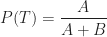
All project managers want to know whether the projects they’re working on will finish on time. So, as our example, we’ll assume that a project manager asks the question: what’s the probability that my project will finish on time? There are only two possibilties here: either the project finishes on (or before) time or it doesn’t. Let’s express this formally. Denoting the event the project finishes on (or before) time by 


Equation (1) is simply a statement of the fact that the sum of the probabilities of all possible outcomes must equal 1.
Fig 1. is a pictorial representation of the two events and how they relate to the entire universe of projects done by the organisation our project manager works in. The rectangular areas 


Fig 1: On Time and Not on Time projects
In terms of areas, the probabilities quoted above can be expressed as:
and
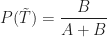
This also makes explicit the fact that the sum of the two probabilities must add up to one.
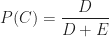
Now, there are several variables that can affect project completion time. Let’s look at just one of them: scope change. Let’s denote the event “there is a major change of scope” by 

Again, since the two possibilities cover the entire spectrum of outcomes, we have:

Fig 2. is a pictorial representation of by

Fig 2: "Major Change" and "No Major Change" projects
The rectangular areas 

and
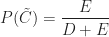
Clearly we also have 
Now things get interesting. One could ask the question: What is the probability of finishing on time given that there has been a major scope change? This is a conditional probability because it represents the likelihood that something will happen (on-time completion) on the condition that something else has already happened (scope change).
As a first step to answering the question posed in the previous paragraph, let’s combine the two events graphically. Fig 3 is a combination of Figs 1 and 2. It shows four possible events:
- On Time with Major Change (
in Fig 3.
- On Time with No Major Change (
in Fig 3.
- Not On Time with Major Change (
in Fig 3.
- Not On Time with No Major Change (
in Fig 3.

Fig 3: Combination of events shown in Figs 1 and 2
We’re interested in the probability that the project finishes on time given that it has suffered a major change in scope. In the notation of conditional probability, this is denoted by 

since 
Similarly, the conditional probability that a project has undergone a major change given that it has come in on time, 
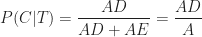
since 
Now, what I’m about to do next may seem like pointless algebraic jugglery, but bear with me…
Consider the ratio of the area

This is simply multiplying and dividing by the same factor (
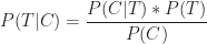
Written in the notation of conditional probabilities, the second and third expressions in (9) are:

which is Bayes theorem.
From the above discussion, it should be clear that Bayes theorem follows from the definition of conditional probability.
We can rewrite Bayes theorem in several equivalent ways:
or
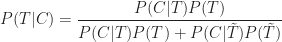
where the denominator in (12) follows from the fact that a project that undergoes a major change will either be on time or will not be on time (there is no other possibility).
A numerical example
To complete the discussion, let’s look at a numerical example.
Assume our project manager has historical data on projects that have been carried out within the organisation. On analyzing the data, the PM finds that 60% of all projects finished on time. This implies:

and

Let us assume that our organisation also tracks major changes made to projects in progress. Say 50% of all historical projects are found to have major changes. This implies:

Finally, let us assume that our project manager has access to detailed data on successful projects, and that an analysis of this data shows that 30% on time projects have undergone at least one major scope change. This gives:

Equations (13) through (16) give us the numbers we need to calculated 
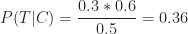
So, in this organisation, if a project undergoes a major change then there’s a 36% probability that it will finish on time. Compare this to the 60% (unconditional) probability of finishing on time. Bayes theorem enables the project manager to quantify the impact of change in scope on project completion time, providing the relevant historical data is available. The italicised bit in the previous sentence is important; I’ll have more to say about it in the concluding section.
In closing this section I should emphasise that although my discussion of Bayes theorem is couched in terms of project completion times and scope changes, the arguments used are general. Bayes theorem holds for any pair of events.
Concluding remarks
It should be clear that the probability calculated in the previous section is an extrapolation based on past experience. In this sense, Bayes Theorem is a formal statement of the belief that one can predict the future based on past events. This goes beyond probability theory; it is an assumption that underlies much of science. It is important to emphasise that the prediction is based on enumeration, not analysis: it is solely based on ratios of the number of projects in one category versus the other; there is no attempt at finding a causal connection between the events of interest. In other words, Bayes theorem suggests there is a correlation between major changes in scope and delays, but it does not tell us why. The latter question can be answered only via a detailed study which might culminate in a theory that explains the causal connection between changes in scope and completion times.
It is also important to emphasise that data used in calculations should be based on events that akin to the one at hand. In the case of the example, I have assumed that historical data is for projects that resemble the one the project manager is working on. This assumption must be validated because there could be situations in which a major change in scope actually reduces completion time (when the project is “scoped-down”, for instance). In such cases, one would need to ensure that the numbers that go into Bayes theorem are based on historical data for “scoped-down” projects only.
To sum up: Bayes theorem expresses a fundamental relationship between conditional probabilities of two events. Its main utility is that it enables us to make probabilistic predictions based on past events; something that a project manager needs to do quite often. In this post I’ve attempted to provide a straightforward explanation of Bayes theorem – how it comes about and what its good for. I hope I’ve succeeded in doing so. But if you’ve found my explanation confusing, I can do no better than to direct you to a couple of excellent references.
Recommended Reading
- An Intuitive (and short) explanation of Bayes Theorem – this is an excellent and concise explanation by Kalid Azad of Better Explained.
- An intuitive explanation of Bayes Theorem – this article by Eliezer Yudkowsky is the best explanation of Bayes theorem I’ve come across. However, it is very long, even by my verbose standards!
Communicating risks using the Improbability Scale
It can be hard to develop an intutitive feel for a probability that is expressed in terms of a single number. The main reason for this is that a numerical probability, without anything to compare it to, may not convey a sense of how likely (or unlikely) an event is. For example, the NSW Road Transport Authority tells us that 0.97% of the registered vehicles on the road in NSW in 2008 were involved in at least one accident. Based on this, the probability that a randomly chosen vehicle will be involved in an accident over a period of one year is 0.0097. Although this number suggests the risk is small, it begs the question: how small? How does it compare to the probability of other, known events? In a short paper entitled, The Improbability Scale, David Ritchie outlines how to make this comparison in an inituitively appealing way.
Ritchie defines the Improbability Scale, 

where 
By definition, 
Let’s look at the improbability of some events expressed in terms of
- Rolling a six on the throw of a die.
- Picking a specific card (say the 10 of diamonds) from a pack (wildcards excluded).
- A (particular) vehicle being involved in at least one accident in the Australian state of NSW over a period of one year (the example quoted in the in the first paragraph).
- One’s birthday occurring on a randomly picked day of the year.
- Probability of getting 10 heads in 10 consecutive coin tosses.
(or 0.00098 );
- Drawing 5 sequential cards of the same suit from a complete deck (a straight flush).
- Being struck by lightning in Australia.
- Winning the Oz Lotto Jackpot.
;
Apart from clarifying the risk of a traffic accident, this tells me (quite unambiguously!) that I must stop buying lottery tickets.
A side benefit of the improbability scale is that it eases the tasks of calculating the probability of combined events. If two events are independent, the probability that they will occur together is given by the product of their individual probabilities of occurrence. Since the logarithm of a product of two number equals the sum of the numbers,
In short: the improbability scale offers a nice way to understand the likelihood of an event occuring in comparison to other events. In particular, the examples discussed above show how it can be used to illustrate and communicate the likelihood of risks in a vivid and intuitive manner.
The failure of risk management: a book review
Introduction
Any future-directed activity has a degree of uncertainty, and uncertainty implies risk. Bad stuff happens – anticipated events don’t unfold as planned and unanticipated events occur. The main function of risk management is to deal with this negative aspect of uncertainty. The events of the last few years suggest that risk management as practiced in many organisations isn’t working. A book by Douglas Hubbard entitled, The Failure of Risk Management – Why it’s Broken and How to Fix It, discusses why many commonly used risk management practices are flawed and what needs to be done to fix them. This post is a summary and review of the book.
Interestingly, Hubbard began writing the book well before the financial crisis of 2008 began to unfold. So although he discusses matters pertaining to risk management in finance, the book has a much broader scope. For instance, it will be of interest to project and program/portfolio management professionals because many of the flawed risk management practices that Hubbard mentions are often used in project risk management.
The book is divided into three parts: the first part introduces the crisis in risk management; the second deals with why some popular risk management practices are flawed; the third discusses what needs to be done to fix these. My review covers the main points of each section in roughly the same order as they appear in the book.
The crisis in risk management
There are several risk management methodologies and techniques in use ; a quick search will reveal some of them. Hubbard begins his book by asking the following simple questions about these:
- Do these risk management methods work?
- Would any organisation that uses these techniques know if they didn’t work?
- What would be the consequences if they didn’t work
His contention is that for most organisations the answers to the first two questions are negative. To answer the third question, he gives the example of the crash of United Flight 232 in 1989. The crash was attributed to the simultaneous failure of three independent (and redundant) hydraulic systems. This happened because the systems were located at the rear of the plane and debris from a damaged turbine cut lines to all them. This is an example of common mode failure – a single event causing multiple systems to fail. The probability of such an event occurring was estimated to be less than one in a billion. However, the reason the turbine broke up was that it hadn’t been inspected properly (i.e. human error). The probability estimate hadn’t considered human oversight, which is way more likely than one-in-billion. Hubbard uses this example to make the point that a weak risk management methodology can have huge consequences.
Following a very brief history of risk management from historical times to the present, Hubbard presents a list of common methods of risk management. These are:
- Expert intuition – essentially based on “gut feeling”
- Expert audit – based on expert intuition of independent consultants. Typically involves the development of checklists and also uses stratification methods (see next point)
- Simple stratification methods – risk matrices are the canonical example of stratification methods.
- Weighted scores – assigned scores for different criteria (scores usually assigned by expert intuition), followed by weighting based on perceived importance of each criterion.
- Non-probabilistic financial analysis –techniques such as computing the financial consequences of best and worst case scenarios
- Calculus of preferences – structured decision analysis techniques such as multi-attribute utility theory and analytic hierarchy process. These techniques are based on expert judgements. However, in cases where multiple judgements are involved these techniques ensure that the judgements are logically consistent (i.e. do not contradict the principles of logic).
- Probabilistic models – involves building probabilistic models of risk events. Probabilities can be based on historical data, empirical observation or even intuition. The book essentially builds a case for evaluating risks using probabilistic models, and provides advice on how these should be built
The book also discusses the state of risk management practice (at the end of 2008) as assessed by surveys carried out by The Economist, Protiviti and Aon Corporation. Hubbard notes that the surveys are based largely on self-assessments of risk management effectiveness. One cannot place much confidence in these because self-assessments of risk are subject to well known psychological effects such as cognitive biases (tendencies to base judgements on flawed perceptions) and the Dunning-Kruger effect (overconfidence in one’s abilities). The acid test for any assessment is whether or not it use sound quantitative measures. Many of the firms surveyed fail on this count: they do not quantify risks as well as they claim they do. Assigning weighted scores to qualitative judgements does not count as a sound quantitative technique – more on this later.
So, what are some good ways of measuring the effectiveness of risk management? Hubbard lists the following:
- Statistics based on large samples – the use of this depends on the availability of historical or other data that is similar to the situation at hand.
- Direct evidence – this is where the risk management technique actually finds some problem that would not have been found otherwise. For example, an audit that unearths dubious financial practices
- Component testing – even if one isn’t able to test the method end-to-end, it may be possible to test specific components that make up the method. For example, if the method uses computer simulations, it may be possible to validate the simulations by applying them to known situations.
- Check of completeness – organisations need to ensure that their risk management methods cover the entire spectrum of risks, else there’s a danger that mitigating one risk may increase the probability of another. Further, as Hubbard states, “A risk that’s not even on the radar cannot be managed at all.” As far as completeness is concerned, there are four perspectives that need to be taken into account. These are:
- Internal completeness – covering all parts of the organisation
- External completeness – covering all external entities that the organisation interacts with.
- Historical completeness – this involves covering worst case scenarios and historical data.
- Combinatorial completeness – this involves considering combinations of events that may occur together; those that may lead to common-mode failure discussed earlier.
Finally, Hubbard closes the first section with the observation that it is better not to use any formal methodology than to use one that is flawed. Why? Because a flawed methodology can lead to an incorrect decision being made with high confidence.
Why it’s broken
Hubbard begins this section by identifying the four major players in the risk management game. These are:
- Actuaries: These are perhaps the first modern professional risk managers. They use quantitative methods to manage risks in the insurance and pension industry. Although the methods actuaries use are generally sound, the profession is slow to pick up new techniques. Further, many investment decisions that insurance companies do not come under the purview of actuaries. So, actuaries typically do not cover the entire spectrum of organizational risks.
- Physicists and mathematicians: Many rigorous risk management techniques came out of statistical research done during the second world war. Hubbard therefore calls this group War Quants. One of the notable techniques to come out of this effort is the Monte Carlo Method – originally proposed by Nick Metropolis, John Neumann and Stanislaw Ulam as a technique to calculate the averaged trajectories of neutrons in fissile material (see this article by Nick Metropolis for a first-person account of how the method was developed). Hubbard believes that Monte Carlo simulations offer a sound, general technique for quantitative risk analysis. Consequently he spends a fair few pages discussing these methods, albeit at a very basic level. More about this later.
- Economists: Risk analysts in investment firms often use quantitative techniques from economics. Popular techniques include modern portfolio theory and models from options theory (such as the Black-Scholes model) . The problem is that these models are often based on questionable assumptions. For example, the Black-Scholes model assumes that the rate of return on a stock is normally distributed (i.e. its value is lognormally distributed) – an assumption that’s demonstrably incorrect as witnessed by the events of the last few years . Another way in which economics plays a role in risk management is through behavioural studies, in particular the recognition that decisions regarding future events (be they risks or stock prices) are subject to cognitive biases. Hubbard suggests that the role of cognitive biases in risk management has been consistently overlooked. See my post entitled Cognitive biases as meta-risks and its follow-up for more on this point.
- Management consultants: In Hubbard’s view, management consultants and standards institutes are largely responsible for many of the ad-hoc approaches to risk management. A particular favourite of these folks are ad-hoc scoring methods that involve ordering of risks based on subjective criteria. The scores assigned to risks are thus subject to cognitive bias. Even worse, some of the tools used in scoring can end up ordering risks incorrectly. Bottom line: many of the risk analysis techniques used by consultants and standards have no justification.
Following the discussion of the main players in the risk arena, Hubbard discusses the confusion associated with the definition of risk. There are a plethora of definitions of risk, most of which originated in academia. Hubbard shows how some of these contradict each other while others are downright non-intuitive and incorrect. In doing so, he clarifies some of the academic and professional terminology around risk. As an example, he takes exception to the notion of risk as a “good thing” – as in the PMI definition, which views risk as “an uncertain event or condition that, if it occurs, has a positive or negative effect on a project objective.” This definition contradicts common (dictionary) usage of the term risk (which generally includes only bad stuff). Hubbard’s opinion on this may raise a few eyebrows (and hackles!) in project management circles, but I reckon he has a point.
In my opinion, the most important sections of the book are chapters 6 and 7, where Hubbard discusses why “expert knowledge and opinions” (favoured by standards and methodologies are flawed) and why a very popular scoring method (risk matrices) is “worse than useless.” See my posts on the limitations of scoring techniques and Cox’s risk matrix theorem for detailed discussions of these points.
A major problem with expert estimates is overconfidence. To overcome this, Hubbard advocates using calibrated probability assessments to quantify analysts’ abilities to make estimates. Calibration assessments involve getting analysts to answer trivia questions and eliciting confidence intervals for each answer. The confidence intervals are then checked against the proportion of correct answers. Essentially, this assesses experts’ abilities to estimates by tracking how often they are right. It has been found that people can improve their ability to make subjective estimates through calibration training – i.e. repeated calibration testing followed by feedback. See this site for more on probability calibration.
Next Hubbard tackles several “red herring” arguments that are commonly offered as reasons not to manage risks using rigorous quantitative methods. Among these are arguments that quantitative risk analysis is impossible because:
- Unexpected events cannot be predicted.
- Risks cannot be measured accurately.
Hubbard states that the first objection is invalid because although some events (such as spectacular stockmarket crashes) may have been overlooked by models, it doesn’t prove that quantitative risk as a whole is flawed. As he discusses later in the book, many models go wrong by assuming Gaussian probability distributions where fat-tailed ones would be more appropriate. Of course, given limited data it is difficult to figure out which distribution’s the right one. So, although Hubbard’s argument is correct, it offers little comfort to the analyst who has to model events before they occur.
As far as the second is concerned, Hubbard has written another book on how just about any business variable (even intangible ones) can be measured. The book makes a persuasive case that most quantities of interest can be measured, but there are difficulties. First, figuring out the factors that affect a variable is not a straightforward task. It depends, among other things, on the availability of reliable data, the analyst’s experience etc. Second, much depends on the judgement of the analyst, and such judgements are subject to bias. Although calibration may help reduce certain biases such as overconfidence, it is by no means a panacea for all biases. Third, risk-related measurements generally involve events that are yet to occur. Consequently, such measurements are based on incomplete information. To make progress one often has to make additional assumptions which may not justifiable a priori.
Hubbard is a strong advocate for quantitative techniques such as Monte Carlo simulations in managing risks. However, he believes that they are often used incorrectly. Specifically:
- They are often used without empirical data or validation – i.e. their inputs and results are not tested through observation.
- Are generally used piecemeal – i.e. used in some parts of an organisation only, and often to manage low-level, operational risks.
- They frequently focus on variables that are not important (because these are easier to measure) rather than those that are important. Hubbard calls this perverse occurrence measurement inversion. He contends that analysts often exclude the most important variables because these are considered to be “too uncertain.”
- They use inappropriate probability distributions. The Normal distribution (or bell curve) is not always appropriate. For example, see my posts on the inherent uncertainty of project task estimates for an intuitive discussion of the form of the probability distribution for project task durations.
- They do not account for correlations between variables. Hubbard contends that many analysts simply ignore correlations between risk variables (i.e. they treat variables as independent when they actually aren’t). This almost always leads to an underestimation of risk because correlations can cause feedback effects and common mode failures.
Hubbard dismisses the argument that rigorous quantitative methods such as Monte Carlo are “too hard.” I agree, the principles behind Monte Carlo techniques aren’t hard to follow – and I take the opportunity to plug my article entitled An introduction to Monte Carlo simulations of project tasks 🙂 . As far as practice is concerned, there are several commercially available tools that automate much of the mathematical heavy-lifting. I won’t recommend any, but a search using the key phrase monte carlo simulation tool will reveal many.
How to Fix it
The last part of the book outlines Hubbard’s recommendations for improving the practice of risk management. Most of the material presented here draws on the previous section of the book. His main suggestions are to:
- Adopt the language, tools and philosophy of uncertain systems. To do this he recommends:
- Using calibrated probabilities to express uncertainties. Hubbard believes that any person who makes estimates that will be used in models should be calibrated. He offers some suggestions on people can improve their ability to estimate through calibration – discussed earlier and on this web site.
- Employing quantitative modelling techniques to model risks. In particular, he advocates the use of Monte Carlo methods to model risks. He also provides a list of commercially available PC-based Monte Carlo tools. Hubbard makes the point that modelling forces analysts to decompose the systems of interest and understand the relationships between their components (see point 2 below).
- Developing an understanding of the basic rules of probability including independent events, conditional probabilities and Bayes’ Theorem. He gives examples of situations in which these rules can help analysts extrapolate
To this, I would also add that it is important to understand the idea that an estimate isn’t a number, but a probability distribution – i.e. a range of numbers, each with a probability attached to it.
- Build, validate and test models using reality as the ultimate arbiter. Models should be built iteratively, testing each assumption against observation. Further, models need to incorporate mechanisms (i.e. how and why the observations are what they are), not just raw observations. This is often hard to do, but at the very least models should incorporate correlations between variables. Note that correlations are often (but not always!) indicative of an underlying mechanism. See this post for an introductory example of Monte Carlo simulation involving correlated variables.
- Lobbying for risk management to be given appropriate visibility in organisation.s
In the penultimate chapter of the book, Hubbard fleshes out the characteristics or traits of good risk analysts. As he mentions several times in the book, risk analysis is an empirical science – it arises from experience. So, although the analytical and mathematical (modelling) aspects of risk are important, a good analyst must, above all, be an empiricist – i.e. believe that knowledge about risks can only come from observation of reality. In particular, tesing models by seeing how well they match historical data and tracking model predictions are absolutely critical aspects of a risk analysts job. Unfortunately, many analysts do not measure the performance of their risk models. Hubbard offers some excellent suggestions on how analysts can refine and improve their models via observation.
Finally, Hubbard emphasises the importance of creating an organisation-wide approach to managing risks. This ensures that organisations will tackle the most important risks first, and that its risk management budgets will be spent in the most effective way. Many of the tools and approaches that he suggests in the book are most effective if they are used in a consistent way across the entire organisation. In reality, though, risk management languishes way down in the priorities of senior executives. Even those who profess to understanding the importance of managing risks in a rigorous way, rarely offer risk managers the organisational visibility and support they need to do their jobs.
Conclusion
Whew, that was quite a bit to go through, but for me it was was worth it. Hubbard’s views impelled me to take a closer look at the foundations of project risk management and I learnt a great deal from doing so. Regular readers of this blog would have noticed that I have referenced the book (and some of the references therein) in a few of my articles on risk analysis.
I should add that I’ve never felt entirely comfortable with the risk management approaches advocated by project management methodologies. Hubbard’s book articulates these shortcomings and offers solutions to fix them. Moreover, he does so in a way that is entertaining and accessible. If there is a gap, it is that he does does not delve into the details of model building, but then his other book deals with this in some detail.
To summarise: the book is a must read for anyone interested in risk management. It is especially recommended for project professionals who manage risks using methods that are advocated by project management standards and methodologies.


