Archive for the ‘Statistics’ Category
Fooled by conditionality
Conditional probability refers to the chance that an event will occur given that another (possibly related) event has occurred. Understanding how conditional probability works is important – and occasionally even a matter of life or death. For instance, a person may want to know the chance that she has a life-threatening disease given that she has tested positive for it.
Unfortunately, there is a good deal of confusion about conditional probability. I’m amongst the confused, so I thought I’d do some reading on the topic. I began with the Wikipedia article (which wasn’t too helpful) and then went on to other references. My search lead me to some interesting research papers on the confusion surrounding conditional probabilities. This post is inspired by a couple of papers I came across.
In a paper on the use and misuse of conditional probabilities, Walter Kramer and Gerd Gigerenzer point out that many doctors cannot answer the “life or death” question that I posed in the first paragraph of this post. Here are a few pertinent lines from from their article:
German medical doctors with an average of 14 years of professional experience were asked to imagine using a certain test to screen for colorectal cancer. The prevalence of this type of cancer was 0.3%, the sensitivity of the test (the conditional probability of detecting cancer when there is one) was 50% and the false positive rate was 3%. The doctors were asked: “What is the probability that someone who tests positive actually has colorectal cancer?
Kramer and Gigerenzer found that the doctors’ answers ranged from 1% to 99% with about half of them answering 50% (the sensitivity) or 47% (the sensitivity minus that false positive rate).
You may want to have a try at answering the question before proceeding further.
—
The question can be answered quite easily using Bayes’ rule, which tells us how to calculate the conditional probability of an event given that another (possibly related) event has occurred. If the two events are denoted by A and B, the conditional probability that A will occur given that B has occurred, denoted by P(A|B), is:

Where P(B|A) is the conditional probability that B will occur given that A has occurred and P(A) and P(B) are the probabilities of A and B occurring respectively. See the appendix at the end of this post for more on Bayes rule.
In terms of the problem stated above, Bayes rule is:
P(Has cancer|Tests positive) = P(Tests positive|Has cancer) * P(Has cancer) / P(Tests positive)
From the problem statement we have:
P(Tests positive|Has cancer) =0.5
P(Has cancer) = 0.003
P(Tests positive) = (1-0.003)*0.03 + 0.003*0.5
Note that P(Tests positive) is obtained by noting that a person can test positive in two ways:
- Not having the disease and testing positive.
- Having the disease and testing positive.
Plugging the numbers in, we get:
P(Has cancer|Tests positive) = 0.5 * 0.003 / (0.997*0.03 + 0.003*0.5) = 0.047755
Or about 5%.
Kramer and Gigerenzer contend that the root of the confusion lies in the problem statement: people find it unnatural to reason in terms of probabilities because the terminology of conditional probability is confusing (A given B, B given A – it’s enough to make one’s head spin). To resolve this they recommend stating the problem in terms of frequencies – i.e. number of instances – rather than ratios.
OK, so let’s restate the problem in terms of frequencies (note this is my restatement, not Gigerenzer’s):
Statistically, 3 people in every 1000 have colorectal cancer. We have a test that is 50% accurate. So, out of the 3 people who have the disease, 1.5 of them will test positive for it. The test has a false positive rate of 3%: so about 30 (29.91 actually) of the remaining 997 people who don’t have the disease will test positive. What is the probability that someone who tests positive has the disease?
From the problem restatement we have:
Total number of people who have cancer and test positive in every 1000 = 1.5
Total number of people who test positive in every 1000 = 1.5+30=31.5
P(Have cancer|Test positive) = 1.5/31.5=0.047619
The small difference between the two numbers is due to rounding error (I’ve rounded 29.91 up to 30)
There’s no question that this is much more straightforward.
—
But the story doesn’t end there. In a paper entitled the Non-use of Bayes Rule, Thomas Dohmen and his colleagues Armin Falk,David Huffman, Felix Marklein and Uwe Sunde measured the ability to use Bayesian reasoning (which is academese for “reasoning using Bayes rule”) in a representative sample of the German population. They did so by asking those sampled to answer a question that involved conditional probability. Being aware of Gigerenzer’s work, they stated their question in frequencies rather than probabilities. Here is the question they posed, taken directly from their paper:
Imagine you are on vacation in an area where the weather is mostly sunny and you ask yourself how tomorrow’s weather will be. Suppose that, in the area you are in, on average 90 out of 100 days are sunny, while it rains on 10 out of 100 days. The weather forecast for tomorrow predicts rain. On average, the weather forecast is correct on 80 out of 100 days. What do you think is the probability, in percent, that it is going to rain tomorrow?
Again, you may want to have a go at the problem before proceeding further.
—
The solution is obtained by a straightforward application of Bayes rule which, for the problem above, reads:
P(Rain|Rain forecast)=P(Rain forecast|Rain)* P(Rain) / P(Rain Forecast)
P(Rain forecast|Rain)=0.8 (since there’s an 80% probability of correct forecast)
P(Rain) = 0.1
P(Rain forecast) = P(Rain forecast|Rain)* P(Rain) + P(Rain forecast|Sun)* P(Sun) = 0.8*0.1+0.2*0.9
So, plugging the numbers In , we get P(Rain|Rain forecast)=0.08 / (0.08 + 0.18) = 0.3077 – or approximately 31%.
The surprising thing is that in the study no one got this right, and only 6% of those who were surveyed gave answers within 10% of the correct one.
Dohmen et. al. go on to point out that those with higher education levels – in particular, those with higher degrees were more likely to get the problem wrong! (So it is true: education causes more confusion than clarity.)
Anyway, it appears that stating the problem in terms of frequencies doesn’t help as much as Kramer and Gigerenzer suggest.
In my opinion, whether the problem is stated in terms of frequency or ratio is neither here nor there. The key is to state the problem clearly. In the restatement of the cancer test problem, it isn’t so much the use of frequencies that helps, but that the relevant numbers are presented unambiguously. There is little interpretation required on the problem solver’s part. It is very clear as to what needs to be done; so clear that one does not need to use Bayes rule. In contrast, in the second problem the respondent still has to figure out the individual probabilities that need to be plugged into Bayes’ formula. This requires some interpretation and thought, which doesn’t always come easy. In fact, such reasoning seems to be harder for those with higher degrees than those without. The last paragraph of Dohmen’s paper states:
In a cognitive task as complex as the one we use in this paper, one would expect deliberation cost to be relatively high for people with less formal education. In contrast, for highly educated people deliberation cost should be relatively low. Other things equal, this reasoning would imply that more educated people perform better in assessing conditional probabilities. Our results indicate the contrary, as education, in particular university education, increases the likelihood that respondents are led astray in the probability judgment task. An identification of the exact channels which are responsible for the detrimental effect of education and cognitive ability on Bayesian judgment constitutes a fascinating area for future research.
Fascinating or not, I now have a scapegoat to blame for my being fooled by conditionality.
—-
Appendix: A “derivation” of Bayes Rule
Here’s a quick “derivation” of Bayes rule (the quotes denote that some of the steps in the derivation are a consequence of definitions rather than inferences).
To keep the discussion concrete, we’ll assume that A is the event that a patient has cancer and B the event that a patient tests positive.
The left hand side of Bayes rule, in terms of these events, is:
P(Has cancer|Test positive) = P(Has Cancer & Tests Positive|Tests Positive)
= P(Has cancer & Tests Positive)/P(Tests positive) …..(1)
The second expression in (1) above is merely a restatement of the first. The third is obtained by noting that
P(Has Cancer & Tests positive|Tests positive)= (Number of people who have cancer & test positive)/(Number of people who test positive) …..(2)
and that the probabilities in the numerator and denominator of the third statement in (1) are:
P(Has cancer & Tests positive) = (Number of people who have cancer & test positive)/(Total population sampled) …..(3)
P(Tests positive) = (Number of people who test positive)/(Total population sampled) …..(4)
The third expression in (1) follows from the fact the that the denominators (3) and (4) are identical.
We further note that
P(Has cancer &Tests positive) = [P(Test positive & Has cancer)/P(Has cancer)] * P(Has cancer)
=P(Tests positive|Has Cancer) * P(Has cancer) …..(5)
Here the numerator and denominator have been multiplied by the same factor – P(Has cancer). We have also used the fact that P(Tests positive & Has Cancer)/P(Has cancer) is the same as P(Tests positive|Has cancer).
Substituting (5) in the right hand side of (1), we get:
P(Has cancer|Tests positive) = P(Tests positive|Has cancer) * P(Has cancer) / P(Tests positive)
Which is Bayes rule for this case.
As further reading, I recommend Eliezer Yudkowsky’s brilliant essay, An intuitive explanation of Bayes Theorem.
When more knowledge means more uncertainty – a task correlation paradox and its resolution
Introduction
Project tasks can have a variety of dependencies. The most commonly encountered ones are task scheduling dependencies such as finish-to-start and start-to-start relationships which are available in many scheduling tools. However, other kinds of dependencies are possible too. For example, it can happen that the durations of two tasks are correlated in such a way that if one task takes longer or shorter than average, then so does the other. [Note: In statistics such a relationship between two quantities is called a positive correlation and an inverse relationship is termed a negative correlation]. In the absence of detailed knowledge of the relationship, one can model such duration dependencies through statistical correlation coefficients. In my previous post, I showed – via Monte Carlo simulations – that the uncertainty in the duration of a project increases if project task durations are positively correlated (the increase in uncertainty being relative to the uncorrelated case). At first sight this is counter-intuitive, even paradoxical. Knowing that tasks are correlated essentially amounts to more knowledge about the tasks as compared to the uncorrelated case. More knowledge should equate to less uncertainty, so one would expect the uncertainty to decrease compared to the uncorrelated case. This post discusses the paradox and its resolution using the example presented in the previous post.
I’ll begin with a brief recapitulation of the main points of the previous post and then discuss the paradox in some detail.
The example and the paradox
The “project” that I simulated consisted of two identical, triangularly distributed tasks performed sequentially. The triangular distribution for each of the tasks had the following parameters: minimum, most likely and maximum durations of 2, 4 and 8 days respectively. Simulations were carried out for two cases:
- No correlation between the two tasks.
- A correlation coefficient of 0.79 between the two tasks.
The simulations yielded probability distributions for overall completion times for the two cases. I then calculated the standard deviation for both distributions. The standard deviation is a measure of the “spread” or uncertainty represented by a distribution. The standard deviation for the correlated case turned out to be more than 30% larger than that for the uncorrelated case (2.33 and 1.77 days respectively), indicating that the probability distribution for the correlated case has a much wider spread than that for the uncorrelated case. The difference in spread can be seen quite clearly in figure 5 of my previous post, which depicts the frequency histograms for the two simulations (the frequency histograms are essentially proportional to the probability distribution). Note that the averages for the two cases are 9.34 and 9.32 days – statistically identical, as we might expect, because the tasks are identically distributed.
Why is the uncertainty (as measured by the standard deviation of the distribution) greater in the correlated case?
Here’s a brief explanation why. In the uncorrelated case, the outcome of the first task has no bearing on the outcome of the second. So if the first task takes longer than the average time (or more precisely, median time), the second one would have an even chance of finishing before the average time of the distribution. There is, therefore, a good chance in the uncorrelated case that overruns (underruns) in the first task will be cancelled out by underruns (overruns) in the second. This is essentially why the combined distribution for the uncorrelated case is more symmetric than that of the correlated case (see figure 5 of the previous post). In the correlated case, however, if the first task takes longer than the median time, chances are that the second task will take longer than the median too (with a similar argument holding for shorter-than-median times). The second task thus has an effect of amplifying the outcome of the first task. This effect becomes more pronounced as we move towards the extremes of the distribution, thus making extreme outcomes more likely than in the uncorrelated case. This has the effect of broadening the combined probability distribution – and hence the larger standard deviation.
Now, although the above explanation is technically correct, the sense that something’s not quite right remains: how can it be that knowing more about the tasks that make up a project results in increased overall uncertainty?
Resolving the paradox
The key to resolving the paradox lies in looking at the situation after task A has completed but B is yet to start. Let’s look at this in some detail.
Consider the uncorrelated case first. The two tasks are independent, so after A completes, we still know nothing more about the possible duration of B other than that it is triangularly distributed with min, max and most likely times of 2, 4 and 8 days. In the correlated case, however, the duration of B tracks the duration of A – that is, if A takes a long (or short) time then so will B. So, after A has completed, we have a pretty good idea of how long B will take. Our knowledge of the correlation works to reduce the uncertainty in B – but only after A is done.
One can also frame the argument in terms of conditional probability.
In the uncorrelated case, the probability distribution of B – let’s call it p(B) – is independent of A. So the conditional probability of B given that A has already finished (often denoted as P(B|A)) is identical to P(B). That is, there is no change in our knowledge of B after A has completed. Remember that we know p(B) – it is a triangular distribution with min, max and most likely completion times of 2, 4 and 8 days respectively. In the correlated case, however, P(B|A) is not the same as P(B) – the knowledge that A has completed has a huge bearing on the distribution of B. Even if one does not know the conditional distribution of B, one can say with some certainty that outcomes close to the duration of A are very likely, and outcomes substantially different from A are highly unlikely. The degree of “unlikeliness” – and the consequent shape of the distribution – depends on the value of the correlation coefficient.
Endnote
So we see that, on the one hand, positive correlations between tasks increase uncertainty in the overall duration of the two tasks. This happens because a wider range of outcomes are possible when the tasks are correlated. On the other hand knowledge of the correlation can also reduce uncertainty – but only after one of the correlated tasks is done. There is no paradox here, its all a question of where we are on the project timeline.
Of course, one can argue that the paradox is an artefact of the assumption that the two tasks remain triangularly distributed in the correlated case. It is far from obvious that this assumption is correct, and it is hard to validate in the real world. That said, I should add that most commercially available simulation tools treat correlations in much the same way as I have done in my previous post – see this article from the @Risk knowledge base, for example.
In the end, though, even if the paradox is only an artefact of modelling and has no real world application, it is still a good pedagogic example of how probability distributions can combine to give counter-intuitive results.
Acknowledgement:
Thanks to Vlado Bokan for several interesting conversations relating to this paradox.
The effect of task duration correlations on project schedules – a study using Monte Carlo simulation
Introduction
Some time ago, I wrote a couple of posts on Monte Carlo simulation of project tasks: the the first post presented a fairly detailed introduction to the technique and the second illustrated its use via three simple examples. The examples in the latter demonstrated the effect of various dependencies on overall completion times. The dependencies discussed were: two tasks in series (finish-to-start dependency), two tasks in series with a time delay (finish-to-start dependency with a lag) and two tasks in parallel (start-to-start dependency). All of these are dependencies in timing: i.e. they dictate when a successor task can start in relation to its predecessor. However, there are several practical situations in which task durations are correlated – that is, the duration of one task depends on the duration of another. As an example, a project manager working for an enterprise software company might notice that the longer it takes to elicit requirements the longer it takes to customise the software. When tasks are correlated thus, it is of interest to find out the effect of the correlation on the overall (project) completion time. In this post I explore the effect of correlations on project schedules via Monte Carlo simulation of a simple “project” consisting of two tasks in series.
A bit about what’s coming before we dive into it. I begin with a brief discusssion on how correlations are quantified. I then describe the simulation procedure, following which I present results for the example mentioned earlier, with and without correlations. I then present a detailed comparison of the results for the uncorrelated and correlated cases. It turns out that correlations increase uncertainty. This seemed counter-intuitive to me at first, but the simulations helped me see why it is so.
Note that I’ve attempted to keep the discussion intuitive and (largely) non-mathematical by relying on graphs and tables rather than formulae. There are a few formulae but most of these can be skipped quite safely.
Correlated project tasks
Imagine that there are two project tasks, A and B, which need to be performed sequentially. To keep things simple, I’ll assume that the durations of A and B are described by a triangular distribution with minimum, most likely and maximum completion times of 2, 4 and 8 days respectively (see my introductory Monte Carlo article for a detailed discussion of this distribution – note that I used hours as the unit of time in that post). In the absence of any other information, it is reasonable to assume that the durations of A and B are independent or uncorrelated – i.e. the time it takes to complete task A does not have any effect on the duration of task B. This assumption can be tested if we have historical data. So let’s assume we have the following historical data gathered from 10 projects:
| Duration A (days)) | duration B (days) |
| 2.5 | 3 |
| 3 | 3 |
| 7 | 7.5 |
| 6 | 4.5 |
| 5.5 | 3.5 |
| 4.5 | 4.5 |
| 5 | 5.5 |
| 4 | 4.5 |
| 6 | 5 |
| 3 | 3.5 |
Figure 1 shows a plot of the duration of A vs. the duration of B. The plot suggests that there is a relationship between the two tasks – the longer A takes, the chances are that B will take longer too.

Figure 1: Duration of A vs. Duration of B
In technical terms we would say that A and B are positively correlated (if one decreased as the other increased, the correlation would be negative).
There are several measures of correlation, the most common one being Pearson’s coefficient of correlation 
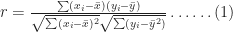
In this case 


The Pearson coefficient, can vary between -1 and 1: the former being a perfect negative correlation and the latter a perfect positive one [Note: The Pearson coefficient is sometimes referred to as the product-moment correlation coefficient]. On calculating
If A and B are correlated as discussed above, simulations which assume the tasks to be independent will not be correct. In the remainder of this article I’ll discuss how correlations affect overall task durations via a Monte Carlo simulation of the aforementioned example.
Simulating correlated project tasks
There are two considerations when simulating correlated tasks. The first is to characterize the correlation accurately. For the purposes of the present discussion I’ll assume that the correlation is described adequately by a single coefficient as discussed in the previous section. The second issue is to generate correlated completion times that satisfy the individual task duration distributions (Remember that the two tasks A and B have completion times that are described by a triangular distribution with minimum, maximum and most likely times of 2, 4 and 8 days). What we are asking for, in effect, is a way to generate a series of two correlated random numbers, each of which satisfy the triangular distribution.
The best known algorithm to generate correlated sets of random numbers in a way that preserves the individual (input) distributions is due to Iman and Conover. The beauty of the Iman-Conover algorithm is that it takes the uncorrelated data for tasks A and B (simulated separately) as input and induces the desired correlation by simply re-ordering the uncorrelated data. Since the original data is not changed, the distributions for A and B are preserved. Although the idea behind the method is simple, it is technically quite complex. The details of the technique aren’t important – but I offer a partial “hand-waving” explanation in the appendix at the end of this post. Fortunately I didn’t have to implement the Iman-Conover algorithm because someone else has done the hard work: Steve Roxburgh has written a graphical tool to generate sets of correlated random variables using the technique (follow this link to download the software and this one to view a brief tutorial) . I used Roxburgh’s utility to generate sets of random variables for my simulations.
I looked at two cases: the first with no correlation between A and B and the second with a correlation of 0.79 between A and B. Each simulation consisted of 10,000 trials – basically I generated two sets of 10,000 triangularly-distributed random numbers, the first with a correlation coefficient close to zero and the second with a correlation coefficient of 0.79. Figures 2 and 3 depict scatter plots of the durations of A vs. the durations of B (for the same trial) for the uncorrelated and correlated cases. The correlation is pretty clear to see in Figure 3.

Figure 2: Scatter plot of duration of A vs. duration of B (uncorrelated)

Figure 3: Scatter plot of duration of A vs. duration of B (correlated)
To check that the generated trials for A and B do indeed satisfy the triangular distribution, I divided the difference between the minimum and maximum times (for the individual tasks) into 0.5 day intervals and plotted the number of trials that fall into each interval. The resulting histograms are shown in Figure 4. Note that the blue and red bars are frequency plots for the case where A and B are uncorrelated and the green and pink (purple?) bars are for the case where they are correlated.

Figure 4: Frequency histograms for A and B (correlated and uncorrelated)
The histograms for all four cases are very similar, demonstrating that they all follow the specified triangular distribution. Figures 2 through 4 give confidence (but do not prove!) that Roxburgh’s utility works as advertised: i.e. that it generates sets of correlated random numbers in a way that preserves the desired distribution.
Now, to simulate A and B in sequence I simply added the durations of the individual tasks for each trial. I did this twice – once each for the correlated and uncorrelated data sets – which yielded two sets of completion times, varying between 4 days (the theoretical minimum) and 16 days (the theoretical maximum). As before, I plotted a frequency histogram for the uncorrelated and correlated case (see Figure 5). Note that the difference in the heights of the bars has no significance – it is an artefact of having the same number of trials (10,000) in both cases. What is significant is the difference in the spread of the two plots – the correlated case has a greater spread signifying an increased probability of very low and very high completion times compared to the uncorrelated case.

Figure 5: Frequency histograms for overall duration (blue=uncorrelated, red=correlated)
Note that the uncorrelated case resembles a Normal distribution – it is more symmetric than the original triangular distribution. This is a consequence of the Central Limit Theorem which states that the sum of identically distributed, independent (i.e. uncorrelated) random numbers is Normally distributed, regardless of the form of original distribution. The correlated distribution, on the other hand, has retained the shape of the original triangular distribution. This is no surprise: the relatively high correlation coefficient ensures that A and B will behave in a similar fashion and, hence, so will their sum.
Figure 6 is a plot of the cumulative distribution function (CDF) for the uncorrelated and correlated cases. The value of the CDFat any time 

Figure 6: Cumulative probability distribution for uncorrelated (blue) and correlated (red) cases
The cumulative distribution clearly shows the greater spread in the correlated case: for small values of 
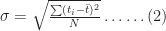
wher 

In both (2) and (3) 
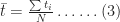
The averages,
So, the simulations tell us that correlations increase uncertainty. Let’s try to understand why this happens. Basically, if tasks are correlated positively, they “track” each other: that is, if one takes a long time so will the other (with the same holding for short durations). The upshot of this is that the overall completion time tends to get “stretched” if the first task takes longer than average whereas it gets “compressed” if the first task finishes earlier than average. Since the net effect of stretching and compressing would balance out, we would expect the mean completion time (or any other measure of central tendency – such as the mode or median) to be relatively unaffected. However, because extremes are amplified, we would expect the spread of the distribution to increase.
Wrap-up
In this post I have highlighted the effect of task correlations on project schedules by comparing the results of simulations for two sequential tasks with and without correlations. The example shows that correlations can increase uncertainty. The mechanism is easy to understand: correlations tend to amplify extreme outcomes, thus increasing the spread in the resulting distribution. The effect of the correlation (compared to the uncorrelated case) can be quantified by comparing the standard deviations of the two cases.
Of course, quantifying correlations using a single number is simplistic – real life correlations have all kinds of complex dependencies. Nevertheless, it is a useful first step because it helps one develop an intuition for what might happen in more complicated cases: in hindsight it is easy to see that (positive) correlations will amplify extremes, but the simple model helped me really see it.
— —
Appendix – more on the Iman-Conover algorithm
Below I offer a hand-waving, half- explanation of how the technique works; those interested in a proper, technical explanation should see this paper by Simon Midenhall.
Before I launch off into my explanation, I’ll need to take a bit of a detour on coefficients of correlation. The title of Iman and Conover’s paper talks about rank correlation which is different from product-moment (or Pearson) correlation discussed in this post. A popular measure of rank correlation is the Spearman coefficient, 

where 
| duration A (days) | duration B (days) | rank A | rank B | rank difference squared |
| 2.5 | 3 | 1 | 1 | 0 |
| 3 | 3 | 2 | 1 | 1 |
| 7 | 7.5 | 10 | 10 | 0 |
| 6 | 4.5 | 8 | 5 | 9 |
| 5.5 | 3.5 | 7 | 3 | 16 |
| 4.5 | 4.5 | 5 | 5 | 0 |
| 5 | 5.5 | 6 | 9 | 9 |
| 4 | 4.5 | 4 | 5 | 1 |
| 6 | 5 | 8 | 8 | 0 |
| 3 | 3.5 | 2 | 3 | 1 |
Note that ties cause the subsequent number to be skipped.
The last column lists the rank differences, 
With that background about the rank correlation, we can now move on to a brief discussion of the Iman-Conover algorithm.
In essence, the Iman-Conover method relies on reordering the set of to-be-correlated variables to have the same rank order as a reference distribution which has the desired correlation. To paraphrase from Midenhall’s paper (my two cents in italics):
Given two samples of n values from known distributions X and Y (the triangular distributions for A and B in this case) and a desired correlation between them (of 0.78), first determine a sample from a reference distribution that has exactly the desired linear correlation (of 0.78). Then re-order the samples from X and Y to have the same rank order as the reference distribution. The output will be a sample with the correct (individual, triangular) distributions and with rank correlation coefficient equal to that of the reference distribution…. Since linear (Pearson) correlation and rank correlation are typically close, the output has approximately the desired correlation structure…
The idea is beautifully simple, but a problem remains. How does one calculate the required reference distribution? Unfortunately, this is a fairly technical affair for which I could not find a simple explanation – those interested in a proper, technical discussion of the technique should see Chapter 4 of Midenhall’s paper or the original paper by Iman and Conover.
For completeness I should note that some folks have criticised the use of the Iman-Conover algorithm on the grounds that it generates rank correlated random variables instead of Pearson correlated ones. This is a minor technicality which does not impact the main conclusion of this post: i.e. that correlations increase uncertainty.


