Peirce, Holmes and a gold chain – an essay on abductive reasoning
“It has long been an axiom of mine that the little things are infinitely the most important.” – Sir Arthur Conan Doyle (A Case of Identity)
The scientific method is a systematic approach to acquiring and establishing knowledge about how the world works. A scientific investigation typically starts with the formulation of a hypothesis – an educated, evidence-based guess about the mechanism behind the phenomenon being studied – and proceeds by testing how well the hypothesis holds up against experiments designed to disconfirm it.
Although many philosophers have waxed eloquent about the scientific method, very few of them have talked about the process of hypothesis generation. Indeed, most scientists will recognise a good hypothesis when they stumble upon one, but they usually will not be able to say how they came upon it. Hypothesis generation is essentially a creative act that requires a deep familiarity with the phenomenon in question and a spark of intuition. The latter is absolutely essential, a point captured eloquently in the following lines attributed to Einstein:
“…[Man] makes this cosmos and its construction the pivot of his emotional life in order to find in this way the peace and serenity which he cannot find in the narrow whirlpool of personal experience. The supreme task is to arrive at those universal elementary laws from which the cosmos can be built up by pure deduction. There is no logical path to these laws; only intuition, resting on sympathetic understanding of experience can reach them…” – quoted from Zen and The Art of Motorcycle Maintenance by Robert Pirsig.
The American philosopher, Charles Peirce, recognised that hypothesis generation involves a special kind of reasoning, one that enables the investigator to zero in on a small set of relevant facts out of an infinity of possibilities.

Charles Sanders Peirce
As Peirce wrote in one of his papers:
“A given object presents an extraordinary combination of characters of which we should like to have an explanation. That there is any explanation of them is a pure assumption; and if there be, it is [a single] fact which explains them; while there are, perhaps, a million other possible ways of explaining them, if they were not all, unfortunately, false.
A man is found in the streets of New York stabbed in the back. The chief of police might open a directory and put his finger on any name and guess that that is the name of the murderer. How much would such a guess be worth? But the number of names in the directory does not approach the multitude of possible laws of attraction which could have accounted for Kepler’s law of planetary motion and, in advance of verification by predications of perturbations etc., would have accounted for them to perfection. Newton, you will say, assumed that the law would be a simple one. But what was that but piling guess on guess? Surely vastly more phenomena in nature are complex than simple…” – quoted from this paper by Thomas Sebeok.
Peirce coined the term abduction (as opposed to induction or deduction) to refer to the creative act of hypothesis generation. In the present day, the term is used to the process of justifying hypotheses rather than generating them (see this article for more on the distinction). In the remainder of this piece I will use the term in its Peircean sense.
–x–
Contrary to what is commonly stated, Arthur Conan Doyle’s fictional detective employed abductive rather than deductive methods in his cases. Consider the following lines, taken from an early paragraph of Sherlock Holmes’ most celebrated exploit, The Adventure of the Speckled Band. We join Holmes in conversation with a lady who has come to him for assistance:

…You have come in by train this morning, I see.”
“You know me, then?”
“No, but I observe the second half of a return ticket in the palm of your left glove. You must have started early, and yet you had a good drive in a dog-cart, along heavy roads, before you reached the station.”
The lady gave a violent start and stared in bewilderment at my companion.
“There is no mystery, my dear madam,” said he, smiling. “The left arm of your jacket is spattered with mud in no less than seven places. The marks are perfectly fresh. There is no vehicle save a dog-cart which throws up mud in that way, and then only when you sit on the left-hand side of the driver.”
“Whatever your reasons may be, you are perfectly correct,” said she. “I started from home before six, reached Leatherhead at twenty past, and came in by the first train to Waterloo…
Notice what Holmes does: he forms hypotheses about what the lady did, based on a selective observation of facts. Nothing is said about why he picks those particular facts – the ticket stub and the freshness / location of mud spatters on the lady’s jacket. Indeed, as Holmes says in another story, “You know my method. It is founded upon the observation of trifles.”
Abductive reasoning is essentially about recognising which trifles are important.
–x–
I have a gold chain that my mum gave me many years ago. I’ve worn it for so long that now I barely notice it. The only time I’m consciously aware that I’m wearing the chain is when I finger it around my neck, a (nervous?) habit I have developed over time.
As you might imagine, I’m quite attached to my gold chain. So, when I discovered it was missing a few days ago, my first reaction was near panic, I felt like a part of me had gone missing.
Since I hardly ever take the chain off, I could not think of any plausible explanation for how I might have lost it. Indeed, the only time I have had to consistently take the chain off is when going in for an X-ray or, on occasion, through airport security.
Where could it have gone?
After mulling over it for a while, the only plausible explanation I could think of is that I had taken it off at airport security when returning from an overseas trip a week earlier, and had somehow forgotten to collect it on the other side. Realising that it would be near impossible to recover it, I told myself to get used to the idea that it was probably gone for good.
That Sunday, I went for a swim. After doing my laps, I went to the side of the pool for my customary shower. Now, anyone who has taken off a rash vest after a swim will know that it can be a struggle. I suspect this is because water trapped between skin and fabric forms a thin adhesive layer (a manifestation of surface tension perhaps?). Anyway, I wrestled the garment over my head and it eventually came free with a snap, generating a spray of droplets that gleamed in reflected light.
Later in the day, I was at the movies. For some reason, when coming out of the cinema, I remembered the rash vest and the flash of droplets. Hmm, I thought, “a gleam of gold….”
…A near forgotten memory: I vaguely recalled a flash of gold while taking of my rash vest in the pool shower some days ago. Was it after my previous swim or the week earlier, I couldn’t be sure. But I distinctly remembered it had bothered me enough to check the floor of the cubicle cursorily. Finding nothing, I had completely forgotten about it and moved on.
Could it have come off there?
As I thought about it some more, possibility turned to plausibility: I was convinced it was what had happened. Although unlikely I would find it there now, it was worth a try on the hope that someone had found the chain and turned it in as lost property.
I stopped over at the pool on my way back from the movies and asked at reception.
“A gold chain? Hmm, I think you may be in luck,” he said, “I was doing an inventory of lost property last week and came across a chain. I was wondering why no one had come in to claim something so valuable.”
“You’re kidding,” I said, incredulous. “You mean you have a gold chain?”
“Yeah, and I’m pretty sure it will still be there unless someone else has claimed it,” he replied. “I’ll have a look in the safe. Can you describe it for me?”
I described it down to the brief inscription on the clasp.
“Wait here,” he said, “I’ll be a sec”
It took longer than that but he soon emerged, chain in hand.
I could not believe my eyes; I had given up on ever recovering it. “Thanks, so much” I said fervently, “you won’t believe how much it means to me to have found this.”
“No worries mate,” he said, smiling broadly. “Happy to have helped.”
–x–
Endnote: in case you haven’t read it yet, I recommend you take ten minutes to read Sherlock Holmes’ finest adventure and abductive masterpiece, The Adventure of the Speckled Band.
Learning, evolution and the future of work
The Janus-headed rise of AI has prompted many discussions about the future of work. Most, if not all, are about AI-driven automation and its consequences for various professions. We are warned to prepare for this change by developing skills that cannot be easily “learnt” by machines. This sounds reasonable at first, but less so on reflection: if skills that were thought to be uniquely human less than a decade ago can now be done, at least partially, by machines, there is no guarantee that any specific skill one chooses to develop will remain automation-proof in the medium-term future.
This begs the question as to what we can do, as individuals, to prepare for a machine-centric workplace. In this post I offer a perspective on this question based on Gregory Bateson’s writings as well as my work and teaching experiences.
Levels of learning
Given that humans are notoriously poor at predicting the future, it should be clear hitching one’s professional wagon to a specific set of skills is not a good strategy. Learning a set of skills may pay off in the short term, but it is unlikely to work in the long run.
So what can one do to prepare for an ambiguous and essentially unpredictable future?
To answer this question, we need to delve into an important, yet oft-overlooked aspect of learning.
A key characteristic of learning is that it is driven by trial and error. To be sure, intelligence may help winnow out poor choices at some stages of the process, but one cannot eliminate error entirely. Indeed, it is not desirable to do so because error is essential for that “aha” instant that precedes insight. Learning therefore has a stochastic element: the specific sequence of trial and error followed by an individual is unpredictable and likely to be unique. This is why everyone learns differently: the mental model I build of a concept is likely to be different from yours.
In a paper entitled, The Logical Categories of Learning and Communication, Bateson noted that the stochastic nature of learning has an interesting consequence. As he notes:
If we accept the overall notion that all learning is in some degree stochastic (i.e., contains components of “trial and error”), it follows that an ordering of the processes of learning can be built upon a hierarchic classification of the types of error which are to be corrected in the various learning processes.
Let’s unpack this claim by looking at his proposed classification:
Zero order learning – Zero order learning refers to situations in which a given stimulus (or question) results in the same response (or answer) every time. Any instinctive behaviour – such as a reflex response on touching a hot kettle – is an example of zero order learning. Such learning is hard-wired in the learner, who responds with the “correct” option to a fixed stimulus every single time. Since the response does not change with time, the process is not subject to trial and error.
First order learning (Learning I) – Learning I is where an individual learns to select a correct option from a set of similar elements. It involves a specific kind of trial and error that is best explained through a couple of examples. The canonical example of Learning I is memorization: Johnny recognises the letter “A” because he has learnt to distinguish it from the 25 other similar possibilities. Another example is Pavlovian conditioning wherein the subject’s response is altered by training: a dog that initially salivates only when it smells food is trained, by repetition, to salivate when it hears the bell.
A key characteristic of Learning I is that the individual learns to select the correct response from a set of comparable possibilities – comparable because the possibilities are of the same type (e.g. pick a letter from the set of alphabets). Consequently, first order learning cannot lead to a qualitative change in the learner’s response. Much of traditional school and university teaching is geared toward first order learning: students are taught to develop the “correct” understanding of concepts and techniques via a repetition-based process of trial and error.
As an aside, note that much of what goes under the banner of machine learning and AI can be also classed as first order learning.
Second order learning (Learning II) – Second order learning involves a qualitative change in the learner’s response to a given situation. Typically, this occurs when a learner sees a familiar problem situation in a completely new light, thus opening up new possibilities for solutions. Learning II therefore necessitates a higher order of trial and error, one that is beyond the ken of machines, at least at this point in time.
Complex organisational problems, such as determining a business strategy, require a second order approach because they cannot be precisely defined and therefore lack an objectively correct solution. Echoing Horst Rittel, solutions to such problems are not true or false, but better or worse.
Much of the teaching that goes on in schools and universities hinders second order learning because it implicitly conditions learners to frame problems in ways that make them amenable to familiar techniques. However, as Russell Ackoff noted, “outside of school, problems are seldom given; they have to be taken, extracted from complex situations…” Two aspects of this perceptive statement bear further consideration. Firstly, to extract a problem from a situation one has to appreciate or make sense of the situation. Secondly, once the problem is framed, one may find that solving it requires skills that one does not possess. I expand on the implications of these points in the following two sections.
Sensemaking and second order learning
In an earlier piece, I described sensemaking as the art of collaborative problem formulation. There are a huge variety of sensemaking approaches, the gamestorming site describes many of them in detail. Most of these are aimed at exploring a problem space by harnessing the collective knowledge of a group of people who have diverse, even conflicting, perspectives on the issue at hand. The greater the diversity, the more complete the exploration of the problem space.
Sensemaking techniques help in elucidating the context in which a problem lives. This refers to the the problem’s environment, and in particular the constraints that the environment imposes on potential solutions to the problem. As Bateson puts it, context is “a collective term for all those events which tell an organism among what set of alternatives [it] must make [its] next choice.” But this begs the question as to how these alternatives are to be determined. The question cannot be answered directly because it depends on the specifics of the environment in which the problem lives. Surfacing these by asking the right questions is the task of sensemaking.
As a simple example, if I request you to help me formulate a business strategy, you are likely to begin by asking me a number of questions such as:
- What kind of business are you in?
- Who are your customers?
- What’s the competitive landscape?
- …and so on
Answers to these questions fill out the context in which the business operates, thus making it possible to formulate a meaningful strategy.
It is important to note that context rarely remains static, it evolves in time. Indeed, many companies faded away because they failed to appreciate changes in their business context: Kodak is a well-known example, there are many more. So organisations must evolve too. However, it is a mistake to think of an organisation and its environment as evolving independently, the two always evolve together. Such co-evolution is as true of natural systems as it is of social ones. As Bateson tells us:
…the evolution of the horse from Eohippus was not a one-sided adjustment to life on grassy plains. Surely the grassy plains themselves evolved [on the same footing] with the evolution of the teeth and hooves of the horses and other ungulates. Turf was the evolving response of the vegetation to the evolution of the horse. It is the context which evolves.
Indeed, one can think of evolution by natural selection as a process by which nature learns (in a second-order sense).
The foregoing discussion points to another problem with traditional approaches to education: we are implicitly taught that problems once solved, stay solved. It is seldom so in real life because, as we have noted, the environment evolves even if the organisation remains static. In the worst case scenario (which happens often enough) the organisation will die if it does not adapt appropriately to changes in its environment. If this is true, then it seems that second-order learning is important not just for individuals but for organisations as a whole. This harks back to notion of the notion of the learning organisation, developed and evangelized by Peter Senge in the early 90s. A learning organisation is one that continually adapts itself to a changing environment. As one might imagine, it is an ideal that is difficult to achieve in practice. Indeed, attempts to create learning organisations have often ended up with paradoxical outcomes. In view of this it seems more practical for organisations to focus on developing what one might call learning individuals – people who are capable of adapting to changes in their environment by continual learning.
Learning to learn
Cliches aside, the modern workplace is characterised by rapid, technology-driven change. It is difficult for an individual to keep up because one has to:
-
- Figure out which changes are significant and therefore worth responding to.
- Be capable of responding to them meaningfully.
The media hype about the sexiest job of the 21st century and the like further fuel the fear of obsolescence. One feels an overwhelming pressure to do something. The old adage about combating fear with action holds true: one has to do something, but the question then is: what meaningful action can one take?
The fact that this question arises points to the failure of traditional university education. With its undue focus on teaching specific techniques, the more important second-order skill of learning to learn has fallen by the wayside. In reality, though, it is now easier than ever to learn new skills on ones own. When I was hired as a database architect in 2004, there were few quality resources available for free. Ten years later, I was able to start teaching myself machine learning using topnotch software, backed by countless quality tutorials in blog and video formats. However, I wasted a lot of time in getting started because it took me a while to get over my reluctance to explore without a guide. Cultivating the habit of learning on my own earlier would have made it a lot easier.
Back to the future of work
When industry complains about new graduates being ill-prepared for the workplace, educational institutions respond by updating curricula with more (New!! Advanced!!!) techniques. However, the complaints continue and Bateson’s notion of second order learning tells us why:
- Firstly, problem solving is distinct from problem formulation; it is akin to the distinction between human and machine intelligence.
- Secondly, one does not know what skills one may need in the future, so instead of learning specific skills one has to learn how to learn
In my experience, it is possible to teach these higher order skills to students in a classroom environment. However, it has to be done in a way that starts from where students are in terms of skills and dispositions and moves them gradually to less familiar situations. The approach is based on David Cavallo’s work on emergent design which I have often used in my consulting work. Two examples may help illustrate how this works in the classroom:
- Many analytically-inclined people think sensemaking is a waste of time because they see it as “just talk”. So, when teaching sensemaking, I begin with quantitative techniques to deal with uncertainty, such as Monte Carlo simulation, and then gradually introduce examples of uncertainties that are hard if not impossible to quantify. This progression naturally leads on to problem situations in which they see the value of sensemaking.
- When teaching data science, it is difficult to comprehensively cover basic machine learning algorithms in a single semester. However, students are often reluctant to explore on their own because they tend to be daunted by the mathematical terminology and notation. To encourage exploration (i.e. learning to learn) we use a two-step approach: a) classes focus on intuitive explanations of algorithms and the commonalities between concepts used in different algorithms. The classes are not lectures but interactive sessions involving lots of exercises and Q&A, b) the assignments go beyond what is covered in the classroom (but still well within reach of most students), this forces them to learn on their own. The approach works: just the other day, my wonderful co-teachers, Alex and Chris, commented on the amazing learning journey of some of the students – so tentative and hesitant at first, but well on their way to becoming confident data professionals.
In the end, though, whether or not an individual learner learns depends on the individual. As Bateson once noted:
Perhaps the best documented generalization in the field of psychology is that, at any given moment, the behavioral characteristics of a mammal, and especially of [a human], depend upon the previous experience and behavior of that individual.
The choices we make when faced with change depend on our individual natures and experiences. Educators can’t do much about the former but they can facilitate more meaningful instances of the latter, even within the confines of the classroom.

An intuitive introduction to support vector machines using R – Part 1
About a year ago, I wrote a piece on support vector machines as a part of my gentle introduction to data science R series. So it is perhaps appropriate to begin this piece with a few words about my motivations for writing yet another article on the topic.
Late last year, a curriculum lead at DataCamp got in touch to ask whether I’d be interested in developing a course on SVMs for them.
My answer was, obviously, an enthusiastic “Yes!”
Instead of rehashing what I had done in my previous article, I thought it would be interesting to try an approach that focuses on building an intuition for how the algorithm works using examples of increasing complexity, supported by visualisation rather than math. This post is the first part of a two-part series based on this approach.
The article builds up some basic intuitions about support vector machines (abbreviated henceforth as SVM) and then focuses on linearly separable problems. Part 2 (to be released at a future date) will deal with radially separable and more complex data sets. The focus throughout is on developing an understanding what the algorithm does rather than the technical details of how it does it.
Prerequisites for this series are a basic knowledge of R and some familiarity with the ggplot package. However, even if you don’t have the latter, you should be able to follow much of what I cover so I encourage you to press on regardless.
<advertisement> if you have a DataCamp account, you may want to check out my course on support vector machines using R. Chapters 1 and 2 of the course closely follow the path I take in this article. </advertisement>
A one dimensional example
A soft drink manufacturer has two brands of their flagship product: Choke (sugar content of 11g/100ml) and Choke-R (sugar content 8g/100 ml). The actual sugar content can vary quite a bit in practice so it can sometimes be hard to figure out the brand given the sugar content. Given sugar content data for 25 samples taken randomly from both populations (see file sugar_content.xls), our task is to come up with a decision rule for determining the brand.
Since this is one-variable problem, the simplest way to discern if the samples fall into distinct groups is through visualisation. Here’s one way to do this using ggplot:
…and here’s the resulting plot:

Figure 1: Sugar content of samples
Note that we’ve simulated a one-dimensional plot by setting all the y values to 0.
From the plot, it is evident that the samples fall into distinct groups: low sugar content, bounded above by the 8.8 g/100ml sample and high sugar content, bounded below by the 10 g/100ml sample.
Clearly, any point that lies between the two points is an acceptable decision boundary. We could, for example, pick 9.1g/100ml and 9.7g/100ml. Here’s the R code with those points added in. Note that we’ve made the points a bit bigger and coloured them red to distinguish them from the sample points.
label=d_bounds$sep, size=2.5,
vjust=2, hjust=0.5, colour=”red”)
And here’s the plot:
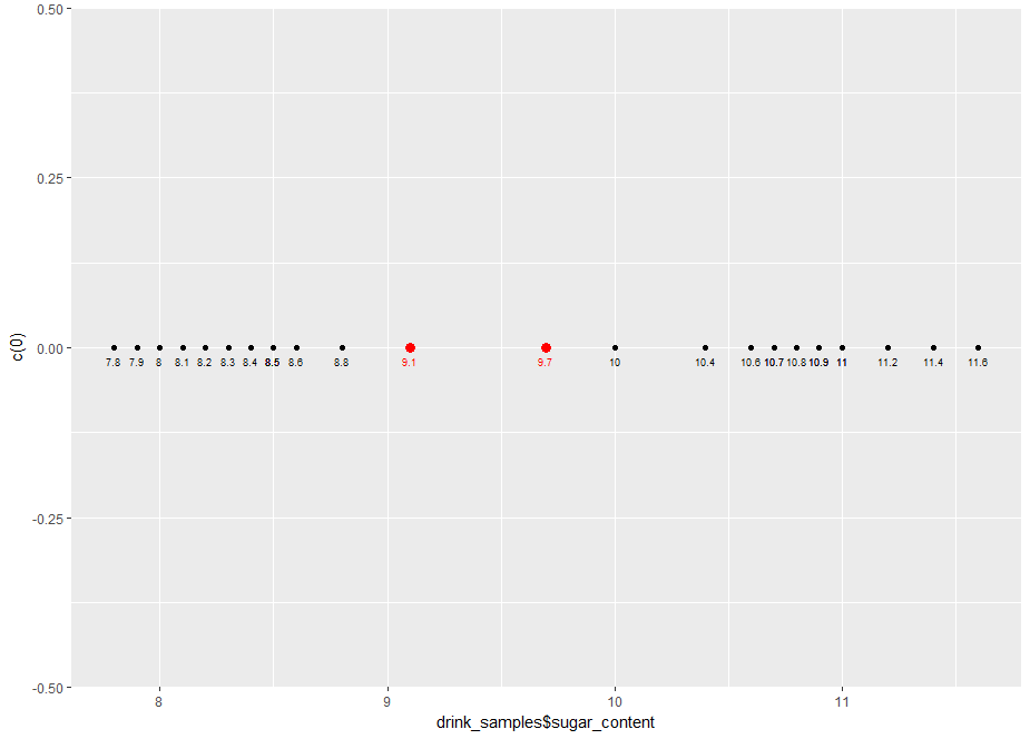
Figure 2: Plot showing example decision boundaries (in red)
Now, a bit about the decision rule. Say we pick the first point as the decision boundary, the decision rule would be:
Say we pick 9.1 as the decision boundary, our classifier (in R) would be:
The other one is left for you as an exercise.
Now, it is pretty clear that although either these points define an acceptable decision boundary, neither of them are the best. Let’s try to formalise our intuitive notion as to why this is so.
The margin is the distance between the points in both classes that are closest to the decision boundary. In case at hand, the margin is 1.2 g/100ml, which is the difference between the two extreme points at 8.8 g/100ml (Choke-R) and 10 g/100ml (Choke). It should be clear that the best separator is the one that lies halfway between the two extreme points. This is called the maximum margin separator. The maximum margin separator in the case at hand is simply the average of the two extreme points:
geom_point(data=mm_sep,aes(x=mm_sep$sep, y=c(0)), colour=”blue”, size=4)
And here’s the plot:
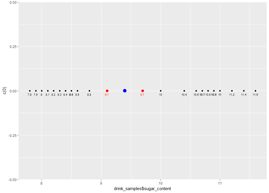
Figure 3: Plot showing maximum margin separator (in blue)
We are dealing with a one dimensional problem here so the decision boundary is a point. In a moment we will generalise this to a two dimensional case in which the boundary is a straight line.
Let’s close this section with some general points.
Remember this is a sample not the entire population, so it is quite possible (indeed likely) that there will be as yet unseen samples of Choke-R and Choke that have a sugar content greater than 8.8 and less than 10 respectively. So, the best classifier is one that lies at the greatest possible distance from both classes. The maximum margin separator is that classifier.
This toy example serves to illustrate the main aim of SVMs, which is to find an optimal separation boundary in the sense described here. However, doing this for real life problems is not so simple because life is not one dimensional. In the remainder of this article and its yet-to-be-written sequel, we will work through examples of increasing complexity so as to develop a good understanding of how SVMs work in addition to practical experience with using the popular SVM implementation in R.
<Advertisement> Again, for those of you who have DataCamp premium accounts, here is a course that covers pretty much the entire territory of this two part series. </Advertisement>
Linearly separable case
The next level of complexity is a two dimensional case (2 predictors) in which the classes are separated by a straight line. We’ll create such a dataset next.
Let’s begin by generating 200 points with attributes x1 and x2, randomly distributed between 0 and 1. Here’s the R code:
Let’s visualise the generated data using a scatter plot:
And here’s the plot
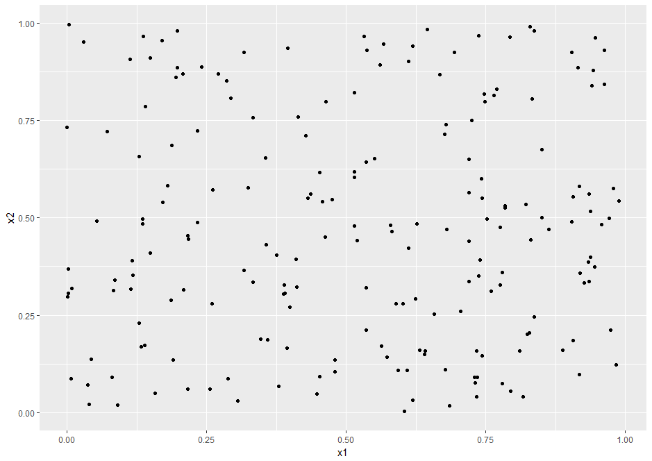
Figure 4: scatter plot of uniformly distributed datapoints
Now let’s classify the points that lie above the line x1=x2 as belonging to the class +1 and those that lie below it as belonging to class -1 (the class values are arbitrary choices, I could have chosen them to be anything at all). Here’s the R code:
Let’s modify the plot in Figure 4, colouring the points classified as +1n blue and those classified -1 red. For good measure, let’s also add in the decision boundary. Here’s the R code:
Note that the parameters in geom_abline() are derived from the fact that the line x1=x2 has slope 1 and y intercept 0.
Here’s the resulting plot:

Figure 5: Linearly separable dataset with boundary.
Next let’s introduce a margin in the dataset. To do this, we need to exclude points that lie within a specified distance of the boundary. A simple way to approximate this is to exclude points that have x1 and x2 values that differ by less a pre-specified value, delta. Here’s the code to do this with delta set to 0.05 units.
The check on the number of datapoints tells us that a number of points have been excluded.
Running the previous ggplot code block yields the following plot which clearly shows the reduced dataset with the depopulated region near the decision boundary:

Figure 6: Dataset with margin (note depleted areas on either side of boundary)
Let’s add the margin boundaries to the plot. We know that these are parallel to the decision boundary and lie delta units on either side of it. In other words, the margin boundaries have slope=1 and y intercepts delta and –delta. Here’s the ggplot code:
And here’s the plot with the margins:

Figure 7: Linearly separable dataset with margin and decision boundary displayed
OK, so we have constructed a dataset that is linearly separable, which is just a short code for saying that the classes can be separated by a straight line. Further, the dataset has a margin, i.e. there is a “gap” so to speak, between the classes. Let’s save the dataset so that we can use it in the next section where we’ll take a first look at the svm() function in the e1071 package.
That done, we can now move on to…
Linear SVMs
Let’s begin by reading in the datafile we created in the previous section:
We then split the data into training and test sets using an 80/20 random split. There are many ways to do this. Here’s one:
The next step is to build the an SVM classifier model. We will do this using the svm() function which is available in the e1071 package. The svm() function has a range of parameters. I explain some of the key ones below, in particular, the following parameters: type, cost, kernel and scale. It is recommended to have a browse of the documentation for more details.
The type parameter specifies the algorithm to be invoked by the function. The algorithm is capable of doing both classification and regression. We’ll focus on classification in this article. Note that there are two types of classification algorithms, nu and C classification. They essentially differ in the way that they penalise margin and boundary violations, but can be shown to lead to equivalent results. We will stick with C classification as it is more commonly used. The “C” refers to the cost which we discuss next.
The cost parameter specifies the penalty to be applied for boundary violations. This parameter can vary from 0 to infinity (in practice a large number compared to 0, say 10^6 or 10^8). We will explore the effect of varying cost later in this piece. To begin with, however, we will leave it at its default value of 1.
The kernel parameter specifies the kind of function to be used to construct the decision boundary. The options are linear, polynomial and radial. In this article we’ll focus on linear kernels as we know the decision boundary is a straight line.
The scale parameter is a Boolean that tells the algorithm whether or not the datapoints should be scaled to have zero mean and unit variance (i.e. shifted by the mean and scaled by the standard deviation). Scaling is generally good practice to avoid undue influence of attributes that have unduly large numeric values. However, in this case we will avoid scaling as we know the attributes are bounded and (more important) we would like to plot the boundary obtained from the algorithm manually.
Building the model is a simple one-line call, setting appropriate values for the parameters:
We expect a linear model to perform well here since the dataset it is linear by construction. Let’s confirm this by calculating training and test accuracy. Here’s the code:
The perfect accuracies confirm our expectation. However, accuracies by themselves are misleading because the story is somewhat more nuanced. To understand why, let’s plot the predicted decision boundary and margins using ggplot. To do this, we have to first extract information regarding these from the svm model object. One can obtain summary information for the model by typing in the model name like so:
kernel = “linear”, scale = FALSE)
Which outputs the following: the function call, SVM type, kernel and cost (which is set to its default). In case you are wondering about gamma, although it’s set to 0.5 here, it plays no role in linear SVMs. We’ll say more about it in the sequel to this article in which we’ll cover more complex kernels. More interesting are the support vectors. In a nutshell, these are training dataset points that specify the location of the decision boundary. We can develop a better understanding of their role by visualising them. To do this, we need to know their coordinates and indices (position within the dataset). This information is stored in the SVM model object. Specifically, the index element of svm_model contains the indices of the training dataset points that are support vectors and the SV element lists the coordinates of these points. The following R code lists these explicitly (Note that I’ve not shown the outputs in the code snippet below):
Let’s use the indices to visualise these points in the training dataset. Here’s the ggplot code to do that:
And here is the plot:

Figure 8: Training dataset showing support vectors
We now see that the support vectors are clustered around the boundary and, in a sense, serve to define it. We will see this more clearly by plotting the predicted decision boundary. To do this, we need its slope and intercept. These aren’t available directly available in the svm_model, but they can be extracted from the coefs, SV and rho elements of the object.
The first step is to use coefs and the support vectors to build the what’s called the weight vector. The weight vector is given by the product of the coefs matrix with the matrix containing the SVs. Note that the fact that only the support vectors play a role in defining the boundary is consistent with our expectation that the boundary should be fully specified by them. Indeed, this is often touted as a feature of SVMs in that it is one of the few classifiers that depends on only a small subset of the training data, i.e. the datapoints closest to the boundary rather than the entire dataset.
Once we have the weight vector, we can calculate the slope and intercept of the predicted decision boundary as follows:
Note that the slope and intercept are quite different from the correct values of 1 and 0 (reminder: the actual decision boundary is the line x1=x2 by construction). We’ll see how to improve on this shortly, but before we do that, let’s plot the decision boundary using the slope and intercept we have just calculated. Here’s the code:
And here’s the augmented plot:
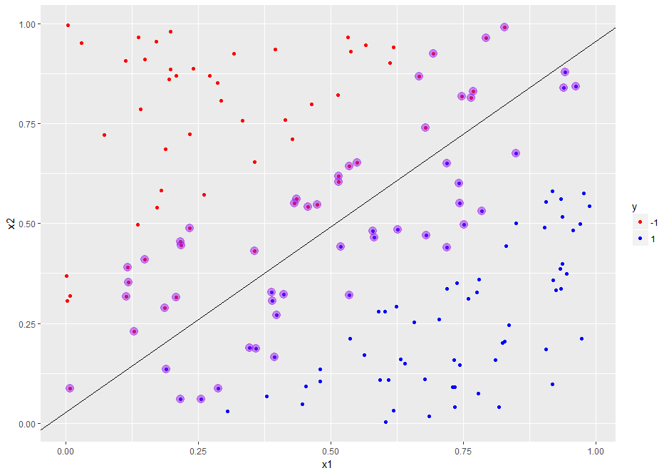
Figure 9: Training dataset showing support vectors and decision boundary
The plot clearly shows how the support vectors “support” the boundary – indeed, if one draws line segments from each of the points to the boundary in such a way that the intersect the boundary at right angles, the lines can be thought of as “holding the boundary in place”. Hence the term support vector.
This is a good time to mention that the e1071 library provides a built-in plot method for svm function. This is invoked as follows:
The svm plot function takes a formula specifying the plane on which the boundary is to be plotted. This is not necessary here as we have only two predictors (x1 and x2) which automatically define a plane.
Here is the plot generated by the above code:
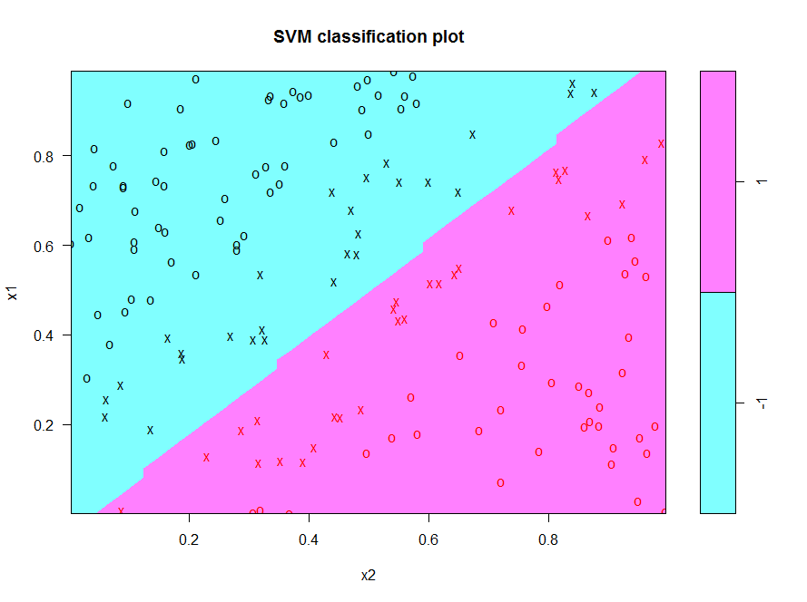
Figure 10: Decision boundary for linearly separable dataset visualised using svm.plot()
Note that the axes are switched (x1 is on the y axis). Aside from that, the plot is reassuringly similar to our ggplot version in Figure 9. Also note that that the support vectors are marked by “x”. Unfortunately the built in function does not display the margin boundaries, but this is something we can easily add to our home-brewed plot. Here’s how. We know that the margin boundaries are parallel to the decision boundary, so all we need to find out is their intercept. It turns out that the intercepts are offset by an amount 1/w[2] units on either side of the decision boundary. With that information in hand we can now write the the code to add in the margins to the plot shown in Figure 9. Here it is:
geom_abline(slope=slope_1,intercept = intercept_1+1/w[2], linetype=”dashed”)
And here is the plot with the margins added in:

Figure 11: Training dataset showing support vectors + decision and margin boundaries
Note that the predicted margins are much wider than the actual ones (compare with Figure 7). As a consequence, many of the support vectors lie within the predicted margin – that is, they violate it. The upshot of the wide margin is that the decision boundary is not tightly specified. This is why we get a significant difference between the slope and intercept of predicted decision boundary and the actual one. We can sharpen the boundary by narrowing the margin. How do we do this? We make margin violations more expensive by increasing the cost. Let’s see this margin-narrowing effect in action by building a model with cost = 100 on the same training dataset as before. Here is the code:
I’ll leave you to calculate the training and test accuracies (as one might expect, these will be perfect).
Let’s inspect the cost=100 model:
kernel = “linear”,cost=100, scale = FALSE)
The number of support vectors is reduced from 55 to 6! We can plot these and the boundary / margin lines using ggplot as before. The code is identical to the previous case (see code block preceding Figure 8). If you run it, you will get the plot shown in Figure 12.
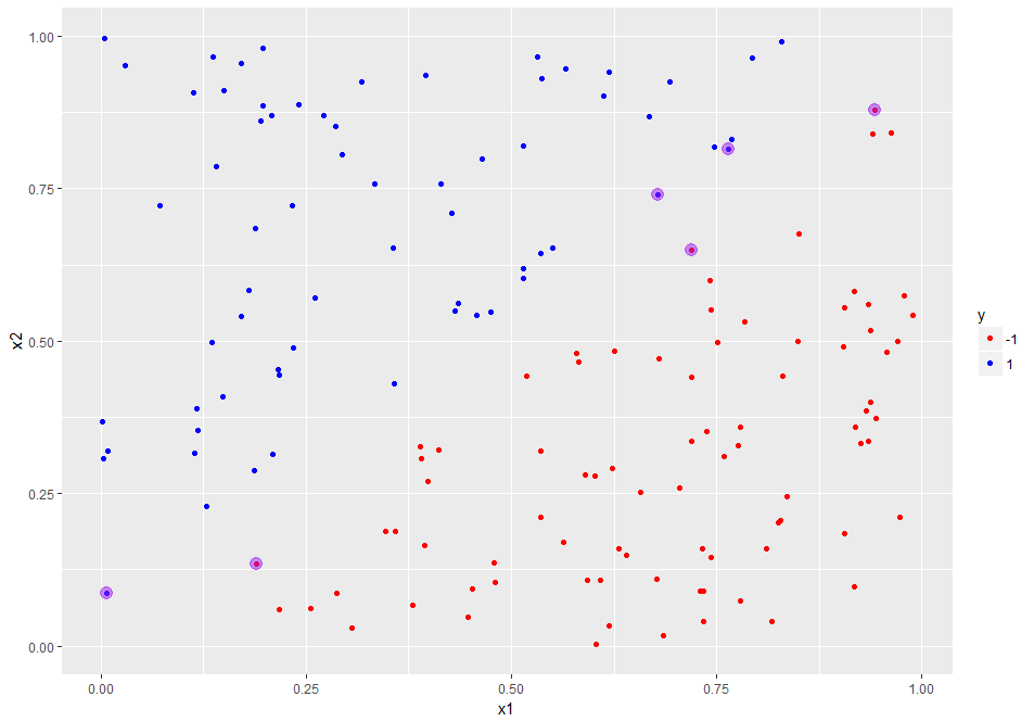
Figure 12: Training dataset showing support vectors for cost=100 case
Since the boundary is more tightly specified, we would expect the slope and intercept of the predicted boundary to be considerably closer to their actual values of 1 and 0 respectively (as compared to the default cost case). Let’s confirm that this is so by calculating the slope and intercept as we did in the code snippets preceding Figure 9. Here’s the code:
Which nicely confirms our expectation.
The decision boundary and margins for the high cost case can also be plotted with the code shown earlier. Her it is for completeness:
geom_abline(slope=slope_100,intercept = intercept_100+1/w[2], linetype=”dashed”)
And here’s the plot:
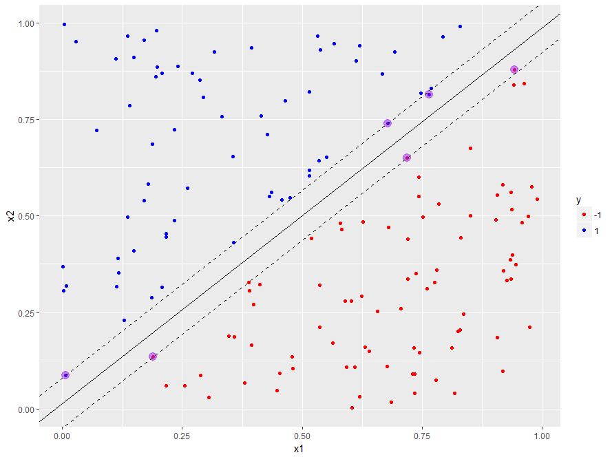
Figure 13: Training dataset with support vectors predicted decision boundary and margins for cost=100
SVMs that allow margin violations are called soft margin classifiers and those that do not are called hard. In this case, the hard margin classifier does a better job because it specifies the boundary more accurately than its soft counterpart. However, this does not mean that hard margin classifier are to be preferred over soft ones in all situations. Indeed, in real life, where we usually do not know the shape of the decision boundary upfront, soft margin classifiers can allow for a greater degree of uncertainty in the decision boundary thus improving generalizability of the classifier.
OK, so now we have a good feel for what the SVM algorithm does in the linearly separable case. We will round out this article by looking at a real world dataset that fortuitously turns out to be almost linearly separable: the famous (notorious?) iris dataset. It is instructive to look at this dataset because it serves to illustrate another feature of the e1071 SVM algorithm – its capability to handle classification problems that have more than 2 classes.
A multiclass problem
The iris dataset is well-known in the machine learning community as it features in many introductory courses and tutorials. It consists of 150 observations of 3 species of the iris flower – setosa, versicolor and virginica. Each observation consists of numerical values for 4 independent variables (predictors): petal length, petal width, sepal length and sepal width. The dataset is available in a standard installation of R as a built in dataset. Let’s read it in and examine its structure:
Now, as it turns out, petal length and petal width are the key determinants of species. So let’s create a scatterplot of the datapoints as a function of these two variables (i.e. project each data point on the petal length-petal width plane). We will also distinguish between species using different colour. Here’s the ggplot code to do this:
And here’s the plot:

Figure 15: iris dataset, petal width vs petal length
On this plane we see a clear linear boundary between setosa and the other two species, versicolor and virginica. The boundary between the latter two is almost linear. Since there are four predictors, one would have to plot the other combinations to get a better feel for the data. I’ll leave this as an exercise for you and move on with the assumption that the data is nearly linearly separable. If the assumption is grossly incorrect, a linear SVM will not work well.
Up until now, we have discussed binary classification problem, i.e. those in which the predicted variable can take on only two values. In this case, however, the predicted variable, Species, can take on 3 values (setosa, versicolor and virginica). This brings up the question as to how the algorithm deals multiclass classification problems – i.e those involving datasets with more than two classes. The SVM algorithm does this using a one-against-one classification strategy. Here’s how it works:
- Divide the dataset (assumed to have N classes) into N(N-1)/2 datasets that have two classes each.
- Solve the binary classification problem for each of these subsets
- Use a simple voting mechanism to assign a class to each data point.
Basically, each data point is assigned the most frequent classification it receives from all the binary classification problems it figures in.
With that said, let’s get on with building the classifier. As before, we begin by splitting the data into training and test sets using an 80/20 random split. Here is the code to do this:
Then we build the model (default cost) and examine it:
The main thing to note is that the function call is identical to the binary classification case. We get some basic information about the model by typing in the model name as before:
kernel = “linear”)
And the train and test accuracies are computed in the usual way:
This looks good, but is potentially misleading because it is for a particular train/test split. Remember, in this case, unlike the earlier example, we do not know the shape of the actual decision boundary. So, to get a robust measure of accuracy, we should calculate the average test accuracy over a number of train/test partitions. Here’s some code to do that:
Which is not too bad at all, indicating that the dataset is indeed nearly linearly separable. If you try different values of cost you will see that it does not make much difference to the average accuracy.
This is a good note to close this piece on. Those who have access to DataCamp premium courses will find that the content above is covered in chapters 1 and 2 of the course on support vector machines in R. The next article in this two-part series will cover chapters 3 and 4.
Summarising
My main objective in this article was to help develop an intuition for how SVMs work in simple cases. We illustrated the basic principles and terminology with a simple 1 dimensional example and then worked our way to linearly separable binary classification problems with multiple predictors. We saw how the latter can be solved using a popular svm implementation available in R. We also saw that the algorithm can handle multiclass problems. All through, we used visualisations to see what the algorithm does and how the key parameters affect the decision boundary and margins.
In the next part (yet to be written) we will see how SVMs can be generalised to deal with complex, nonlinear decision boundaries. In essence, the use a mathematical trick to “linearise” these boundaries. We’ll delve into details of this trick in an intuitive, visual way as we have done here.
Many thanks for reading!


