A gentle introduction to Monte Carlo simulation for project managers
This article covers the why, what and how of Monte Carlo simulation using a canonical example from project management – estimating the duration of a small project. Before starting, however, I’d like say a few words about the tool I’m going to use.
Despite the bad rap spreadsheets get from tech types – and I have to admit that many of their complaints are justified – the fact is, Excel remains one of the most ubiquitous “computational” tools in the corporate world. Most business professionals would have used it at one time or another. So, if you you’re a project manager and want the rationale behind your estimates to be accessible to the widest possible audience, you are probably better off presenting them in Excel than in SPSS, SAS, Python, R or pretty much anything else. Consequently, the tool I’ll use in this article is Microsoft Excel. For those who know about Monte Carlo and want to cut to the chase, here’s the Excel workbook containing all the calculations detailed in later sections. However, if you’re unfamiliar with the technique, you may want to have a read of the article before playing with the spreadsheet.
In keeping with the format of the tutorials on this blog, I’ve assumed very little prior knowledge about probability, let alone Monte Carlo simulation. Consequently, the article is verbose and the tone somewhat didactic.
Introduction
Estimation is key part of a project manager’s role. The most frequent (and consequential) estimates they are asked deliver relate to time and cost. Often these are calculated and presented as point estimates: i.e. single numbers – as in, this task will take 3 days. Or, a little better, as two-point ranges – as in, this task will take between 2 and 5 days. Better still, many use a PERT-like approach wherein estimates are based on 3 points: best, most likely and worst case scenarios – as in, this task will take between 2 and 5 days, but it’s most likely that we’ll finish on day 3. We’ll use three-point estimates as a starting point for Monte Carlo simulation, but first, some relevant background.
It is a truism, well borne out by experience, that it is easier to estimate small, simple tasks than large, complex ones. Indeed, this is why one of the early to-dos in a project is the construction of a work breakdown structure. However, a problem arises when one combines the estimates for individual elements into an overall estimate for a project or a phase thereof. It is that a straightforward addition of individual estimates or bounds will almost always lead to a grossly incorrect estimation of overall time or cost. The reason for this is simple: estimates are necessarily based on probabilities and probabilities do not combine additively. Monte Carlo simulation provides a principled and intuitive way to obtain probabilistic estimates at the level of an entire project based on estimates of the individual tasks that comprise it.
The problem
The best way to explain Monte Carlo is through a simple worked example. So, let’s consider a 4 task project shown in Figure 1. In the project, the second task is dependent on the first, and third and fourth are dependent on the second but not on each other. The upshot of this is that the first two tasks have to be performed sequentially and the last two can be done at the same time, but can only be started after the second task is completed.
To summarise: the first two tasks must be done in series and the last two can be done in parallel.

Figure 1; A project with 4 tasks.
Figure 1 also shows the three point estimates for each task – that is the minimum, maximum and most likely completion times. For completeness I’ve listed them below:
- Task 1 – Min: 2 days; Most Likely: 4 days; Max: 8 days
- Task 2 – Min: 3 days; Most Likely: 5 days; Max: 10 days
- Task 3 – Min: 3 days; Most Likely: 6 days; Max: 9 days
- Task 4 – Min: 2 days; Most Likely: 4 days; Max: 7 days
OK, so that’s the situation as it is given to us. The first step to developing an estimate is to formulate the problem in a way that it can be tackled using Monte Carlo simulation. This bring us to the important topic of the shape of uncertainty aka probability distributions.
The shape of uncertainty
Consider the data for Task 1. You have been told that it most often finishes on day 4. However, if things go well, it could take as little as 2 days; but if things go badly it could take as long as 8 days. Therefore, your range of possible finish times (outcomes) is between 2 to 8 days.
Clearly, each of these outcomes is not equally likely. The most likely outcome is that you will finish the task in 4 days (from what your team member has told you). Moreover, the likelihood of finishing in less than 2 days or more than 8 days is zero. If we plot the likelihood of completion against completion time, it would look something like Figure 2.

Figure 2: Likelihood of finishing on day 2, day 4 and day 8.
Figure 2 begs a couple of questions:
- What are the relative likelihoods of completion for all intermediate times – i.e. those between 2 to 4 days and 4 to 8 days?
- How can one quantify the likelihood of intermediate times? In other words, how can one get a numerical value of the likelihood for all times between 2 to 8 days? Note that we know from the earlier discussion that this must be zero for any time less than 2 or greater than 8 days.
The two questions are actually related. As we shall soon see, once we know the relative likelihood of completion at all times (compared to the maximum), we can work out its numerical value.
Since we don’t know anything about intermediate times (I’m assuming there is no other historical data available), the simplest thing to do is to assume that the likelihood increases linearly (as a straight line) from 2 to 4 days and decreases in the same way from 4 to 8 days as shown in Figure 3. This gives us the well-known triangular distribution.
Jargon Buster: The term distribution is simply a fancy word for a plot of likelihood vs. time.

Figure 3: Triangular distribution fitted to points in Figure 1
Of course, this isn’t the only possibility; there are an infinite number of others. Figure 4 is another (admittedly weird) example.
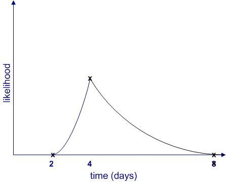
Figure 4: Another distribution that fits the points in Figure 2.
Further, it is quite possible that the upper limit (8 days) is not a hard one. It may be that in exceptional cases the task could take much longer (for example, if your team member calls in sick for two weeks) or even not be completed at all (for example, if she then leaves for that mythical greener pasture). Catering for the latter possibility, the shape of the likelihood might resemble Figure 5.
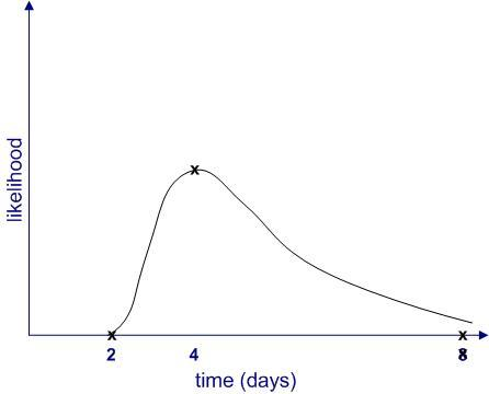
Figure 5: A distribution that allows for a very long (potentially) infinite completion time
The main takeaway from the above is that uncertainties should be expressed as shapes rather than numbers, a notion popularised by Sam Savage in his book, The Flaw of Averages.
[Aside: you may have noticed that all the distributions shown above are skewed to the right – that is they have a long tail. This is a general feature of distributions that describe time (or cost) of project tasks. It would take me too far afield to discuss why this is so, but if you’re interested you may want to check out my post on the inherent uncertainty of project task estimates.
From likelihood to probability
Thus far, I have used the word “likelihood” without bothering to define it. It’s time to make the notion more precise. I’ll begin by asking the question: what common sense properties do we expect a quantitative measure of likelihood to have?
Consider the following:
- If an event is impossible, its likelihood should be zero.
- The sum of likelihoods of all possible events should equal complete certainty. That is, it should be a constant. As this constant can be anything, let us define it to be 1.
In terms of the example above, if we denote time by 


And


Where 


With these assumptions in hand, we can now obtain numerical values for the probability of completion for all times between 2 and 8 days. This can be figured out by noting that the area under the probability curve (the triangle in figure 3 and the weird shape in figure 4) must equal 1, and we’ll do this next. Indeed, for the problem at hand, we’ll assume that all four task durations can be fitted to triangular distributions. This is primarily to keep things simple. However, I should emphasise that you can use any shape so long as you can express it mathematically, and I’ll say more about this towards the end of this article.
The triangular distribution
Let’s look at the estimate for Task 1. We have three numbers corresponding to a minimum, most likely and maximum time. To keep the discussion general, we’ll call these 


Now, what about the probabilities associated with each of these times?
Since 

Figure 6: Triangular distribution redux.
For the simulation, we need to know the equation describing the above distribution. Although Wikipedia will tell us the answer in a mouse-click, it is instructive to figure it out for ourselves. First, note that the area under the triangle must be equal to 1 because the task must finish at some time between

where 
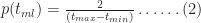
To derive the probability for any time
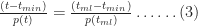
This is a consequence of the fact that the ratios on either side of equation (3) are equal to the slope of the line joining the points 


Figure 7
Substituting (2) in (3) and simplifying a bit, we obtain:
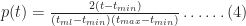

In a similar fashion one can show that the probability for times lying between
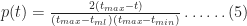

Equations 4 and 5 together describe the probability distribution function (or PDF) for all times between
As it turns out, in Monte Carlo simulations, we don’t directly work with the probability distribution function. Instead we work with the cumulative distribution function (or CDF) which is the probability, 

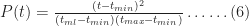
Noting that for 

As expected,
To end this section let’s plug in the numbers quoted by our estimator at the start of this section: 


Figure 8: PDF for triangular distribution (tmin=2, tml=4, tmax=8)

Figure 9 – CDF for triangular distribution (tmin=2, tml=4, tmax=8)
Monte Carlo in a minute
Now with all that conceptual work done, we can get to the main topic of this post: Monte Carlo estimation. The basic idea behind Monte Carlo is to simulate the entire project (all 4 tasks in this case) a large number N (say 10,000) times and thus obtain N overall completion times. In each of the N trials, we simulate each of the tasks in the project and add them up appropriately to give us an overall project completion time for the trial. The resulting N overall completion times will all be different, ranging from the sum of the minimum completion times to the sum of the maximum completion times. In other words, we will obtain the PDF and CDF for the overall completion time, which will enable us to answer questions such as:
- How likely is it that the project will be completed within 17 days?
- What’s the estimated time for which I can be 90% certain that the project will be completed? For brevity, I’ll call this the 90% completion time in the rest of this piece.
“OK, that sounds great”, you say, “but how exactly do we simulate a single task”?
Good question, and I was just about to get to that…
Simulating a single task using the CDF
As we saw earlier, the CDF for the triangular has a S shape and ranges from 0 to 1 in value. It turns out that the S shape is characteristic of all CDFs, regardless of the details underlying PDF. Why? Because, the cumulative probability must lie between 0 and 1 (remember, probabilities can never exceed 1, nor can they be negative).
OK, so to simulate a task, we:
- generate a random number between 0 and 1, this corresponds to the probability that the task will finish at time t.
- find the time, t, that this corresponds to this value of probability. This is the completion time for the task for this trial.
Incidentally, this method is called inverse transform sampling.
An example might help clarify how inverse transform sampling works. Assume that the random number generated is 0.4905. From the CDF for the first task, we see that this value of probability corresponds to a completion time of 4.503 days, which is the completion for this trial (see Figure 10). Simple!
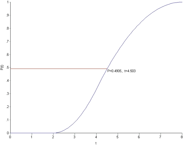
Figure 10: Illustrating inverse transform sampling
In this case we found the time directly from the computed CDF. That’s not too convenient when you’re simulating the project 10,000 times. Instead, we need a programmable math expression that gives us the time corresponding to the probability directly. This can be obtained by solving equations (6) and (7) for

And
(t_{max} - t_{min})} \ldots\ldots(9)](https://s0.wp.com/latex.php?latex=t+%3D+t_%7Bmax%7D+-+%5Csqrt%7B%5B1-P%28t%29%5D%28t_%7Bmax%7D+-%C2%A0+t_%7Bml%7D%29%28t_%7Bmax%7D+-+t_%7Bmin%7D%29%7D+%5Cldots%5Cldots%289%29&bg=ffffff&fg=1c1c1c&s=0&c=20201002)
These can be easily combined in a single Excel formula using an IF function, and I’ll show you exactly how in a minute. Yes, we can now finally get down to the Excel simulation proper and you may want to download the workbook if you haven’t done so already.
The simulation
Open up the workbook and focus on the first three columns of the first sheet to begin with. These simulate the first task in Figure 1, which also happens to be the task we have used to illustrate the construction of the triangular distribution as well as the mechanics of Monte Carlo.
Rows 2 to 4 in columns A and B list the min, most likely and max completion times while the same rows in column C list the probabilities associated with each of the times. For 
Rows 6 through 10005 in column A are simulated probabilities of completion for Task 1. These are obtained via the Excel RAND() function, which generates uniformly distributed random numbers lying between 0 and 1. This gives us a list of probabilities corresponding to 10,000 independent simulations of Task 1.
The 10,000 probabilities need to be translated into completion times for the task. This is done using equations (8) or (9) depending on whether the simulated probability is less or greater than 
Tasks 2-4 are coded in exactly the same way, with distribution parameters in rows 2 through 4 and simulation details in rows 6 through 10005 in the columns listed below:
- Task 2 – probabilities in column D; times in column F
- Task 3 – probabilities in column H; times in column I
- Task 4 – probabilities in column K; times in column L
That’s basically it for the simulation of individual tasks. Now let’s see how to combine them.
For tasks in series (Tasks 1 and 2), we simply sum the completion times for each task to get the overall completion times for the two tasks. This is what’s shown in rows 6 through 10005 of column G.
For tasks in parallel (Tasks 3 and 4), the overall completion time is the maximum of the completion times for the two tasks. This is computed and stored in rows 6 through 10005 of column N.
Finally, the overall project completion time for each simulation is then simply the sum of columns G and N (shown in column O)
Sheets 2 and 3 are plots of the probability and cumulative probability distributions for overall project completion times. I’ll cover these in the next section.
Discussion – probabilities and estimates
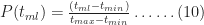
The figure on Sheet 2 of the Excel workbook (reproduced in Figure 11 below) is the probability distribution function (PDF) of completion times. The x-axis shows the elapsed time in days and the y-axis the number of Monte Carlo trials that have a completion time that lie in the relevant time bin (of width 0.5 days). As an example, for the simulation shown in the Figure 11, there were 882 trials (out of 10,000) that had a completion time that lie between 16.25 and 16.75 days. Your numbers will vary, of course, but you should have a maximum in the 16 to 17 day range and a trial number that is reasonably close to the one I got.
Figure 11: Probability distribution of completion times (N=10,000)
I’ll say a bit more about Figure 11 in the next section. For now, let’s move on to Sheet 3 of workbook which shows the cumulative probability of completion by a particular day (Figure 12 below). The figure shows the cumulative probability function (CDF), which is the sum of all completion times from the earliest possible completion day to the particular day.

Figure 12: Probability of completion by a particular day (N=10,000)
To reiterate a point made earlier, the reason we work with the CDF rather than the PDF is that we are interested in knowing the probability of completion by a particular date (e.g. it is 90% likely that we will finish by April 20th) rather than the probability of completion on a particular date (e.g. there’s a 10% chance we’ll finish on April 17th). We can now answer the two questions we posed earlier. As a reminder, they are:
- How likely is it that the project will be completed within 17 days?
- What’s the 90% likely completion time?
Both questions are easily answered by using the cumulative distribution chart on Sheet 3 (or Fig 12). Reading the relevant numbers from the chart, I see that:
- There’s a 60% chance that the project will be completed in 17 days.
- The 90% likely completion time is 19.5 days.
How does the latter compare to the sum of the 90% likely completion times for the individual tasks? The 90% likely completion time for a given task can be calculated by solving Equation 9 for $t$, with appropriate values for the parameters
- Task 1 – 6.5 days
- Task 2 – 8.1 days
- Task 3 – 7.7 days
- Task 4 – 5.8 days
Summing up the first three tasks (remember, Tasks 3 and 4 are in parallel) we get a total of 22.3 days, which is clearly an overestimation. Now, with the benefit of having gone through the simulation, it is easy to see that the sum of 90% likely completion times for individual tasks does not equal the 90% likely completion time for the sum of the relevant individual tasks – the first three tasks in this particular case. Why? Essentially because a Monte Carlo run in which the first three tasks tasks take as long as their (individual) 90% likely completion times is highly unlikely. Exercise: use the worksheet to estimate how likely this is.
There’s much more that can be learnt from the CDF. For example, it also tells us that the greatest uncertainty in the estimate is in the 5 day period from ~14 to 19 days because that’s the region in which the probability changes most rapidly as a function of elapsed time. Of course, the exact numbers are dependent on the assumed form of the distribution. I’ll say more about this in the final section.
To close this section, I’d like to reprise a point I mentioned earlier: that uncertainty is a shape, not a number. Monte Carlo simulations make the uncertainty in estimates explicit and can help you frame your estimates in the language of probability…and using a tool like Excel can help you explain these to non-technical people like your manager.
Closing remarks
We’ve covered a fair bit of ground: starting from general observations about how long a task takes, saw how to construct simple probability distributions and then combine these using Monte Carlo simulation. Before I close, there are a few general points I should mention for completeness…and as warning.
First up, it should be clear that the estimates one obtains from a simulation depend critically on the form and parameters of the distribution used. The parameters are essentially an empirical matter; they should be determined using historical data. The form of the function, is another matter altogether: as pointed out in an earlier section, one cannot determine the shape of a function from a finite number of data points. Instead, one has to focus on the properties that are important. For example, is there a small but finite chance that a task can take an unreasonably long time? If so, you may want to use a lognormal distribution…but remember, you will need to find a sensible way to estimate the distribution parameters from your historical data.
Second, you may have noted from the probability distribution curve (Figure 11) that despite the skewed distributions of the individual tasks, the distribution of the overall completion time is somewhat symmetric with a minimum of ~9 days, most likely time of ~16 days and maximum of 24 days. It turns out that this is a general property of distributions that are generated by adding a large number of independent probabilistic variables. As the number of variables increases, the overall distribution will tend to the ubiquitous Normal distribution.
The assumption of independence merits a closer look. In the case it hand, it implies that the completion times for each task are independent of each other. As most project managers will know from experience, this is rarely the case: in real life, a task that is delayed will usually have knock-on effects on subsequent tasks. One can easily incorporate such dependencies in a Monte Carlo simulation. A formal way to do this is to introduce a non-zero correlation coefficient between tasks as I have done here. A simpler and more realistic approach is to introduce conditional inter-task dependencies As an example, one could have an inter-task delay that kicks in only if the predecessor task takes more than 80% of its maximum time.
Thirdly, you may have wondered why I used 10,000 trials: why not 100, or 1000 or 20,000. This has to do with the tricky issue of convergence. In a nutshell, the estimates we obtain should not depend on the number of trials used. Why? Because if they did, they’d be meaningless.
Operationally, convergence means that any predicted quantity based on aggregates should not vary with number of trials. So, if our Monte Carlo simulation has converged, our prediction of 19.5 days for the 90% likely completion time should not change substantially if I increase the number of trials from ten to twenty thousand. I did this and obtained almost the same value of 19.5 days. The average and median completion times (shown in cell Q3 and Q4 of Sheet 1) also remained much the same (16.8 days). If you wish to repeat the calculation, be sure to change the formulas on all three sheets appropriately. I was lazy and hardcoded the number of trials. Sorry!
Finally, I should mention that simulations can be usefully performed at a higher level than individual tasks. In their highly-readable book, Waltzing With Bears: Managing Risk on Software Projects, Tom De Marco and Timothy Lister show how Monte Carlo methods can be used for variables such as velocity, time, cost etc. at the project level as opposed to the task level. I believe it is better to perform simulations at the lowest possible level, the main reason being that it is easier, and less error-prone, to estimate individual tasks than entire projects. Nevertheless, high level simulations can be very useful if one has reliable data to base these on.
There are a few more things I could say about the usefulness of the generated distribution functions and Monte Carlo in general, but they are best relegated to a future article. This one is much too long already and I think I’ve tested your patience enough. Thanks so much for reading, I really do appreciate it and hope that you found it useful.
Acknowledgement: My thanks to Peter Holberton for pointing out a few typographical and coding errors in an earlier version of this article. These have now been fixed. I’d be grateful if readers could bring any errors they find to my attention.
Risk management and organizational anxiety
In practice risk management is a rational, means-end based process: risks are identified, analysed and then “solved” (or mitigated). Although these steps seem to be objective, each of them involves human perceptions, biases and interests. Where Jill sees an opportunity, Jack may see only risks.
Indeed, the problem of differences in stakeholder perceptions is broader than risk analysis. The recognition that such differences in world-views may be irreconcilable is what led Horst Rittel to coin the now well-known term, wicked problem. These problems tend to be made up of complex interconnected and interdependent issues which makes them difficult to tackle using standard rational- analytical methods of problem solving.
Most high-stakes risks that organisations face have elements of wickedness – indeed any significant organisational change is fraught with risk. Murphy rules; things can go wrong, and they often do. The current paradigm of risk management, which focuses on analyzing and quantifying risks using rational methods, is not broad enough to account for the wicked aspects of risk.
I had been thinking about this for a while when I stumbled on a fascinating paper by Robin Holt entitled, Risk Management: The Talking Cure, which outlines a possible approach to analysing interconnected risks. In brief, Holt draws a parallel between psychoanalysis (as a means to tackle individual anxiety) and risk management (as a means to tackle organizational anxiety). In this post, I present an extensive discussion and interpretation of Holt’s paper. Although more about the philosophy of risk management than its practice, I found the paper interesting, relevant and thought provoking. My hope is that some readers might find it so too.
Background
Holt begins by noting that modern life is characterized by uncertainty. Paradoxically, technological progress which should have increased our sense of control over our surroundings and lives has actually heightened our personal feelings of uncertainty. Moreover, this sense of uncertainty is not allayed by rational analysis. On the contrary, it may have even increased it by, for example, drawing our attention to risks that we may otherwise have remained unaware of. Risk thus becomes a lens through which we perceive the world. The danger is that this can paralyze. As Holt puts it,
…risk becomes the only backdrop to perceiving the world and perception collapses into self-inhibition, thereby compounding uncertainty through inertia.
Most individuals know this through experience: most of us have at one time or another been frozen into inaction because of perceived risks. We also “know” at a deep personal level that the standard responses to risk are inadequate because many of our worries tend to be inchoate and therefore can neither be coherently articulated nor analysed. In Holt’s words:
..People do not recognize [risk] from the perspective of a breakdown in their rational calculations alone, but because of threats to their forms of life – to the non-calculative way they see themselves and the world. [Mainstream risk analysis] remains caught in the thrall of its own ‘expert’ presumptions, denigrating the very lay knowledge and perceptions on the grounds that they cannot be codified and institutionally expressed.
Holt suggests that risk management should account for the “codified, uncodified and uncodifiable aspects of uncertainty from an organizational perspective.” This entails a mode of analysis that takes into account different, even conflicting, perspectives in a non-judgemental way. In essence, he suggests “talking it over” as a means to increase awareness of the contingent nature of risks rather than a means of definitively resolving them.
Shortcomings of risk analysis
The basic aim of risk analysis (as it is practiced) is to contain uncertainty within set bounds that are determined by an organisation’s risk appetite. As mentioned earlier, this process begins by identifying and classifying risks. Once this is done, one determines the probability and impact of each risk. Then, based on priorities and resources available (again determined by the organisation’s risk appetite) one develops strategies to mitigate the risks that are significant from the organisation’s perspective.
However, the messiness of organizational life makes it difficult to see risk in such a clear-cut way. We may pretend to be rational about it, but in reality we perceive it through the lens of our background, interests , experiences. Based on these perceptions we rationalize our action (or inaction!) and simply get on with life. As Holt writes:
The concept [of risk] refers to…the mélange of experience, where managers accept contingencies without being overwhelmed to a point of complete passivity or confusion, Managers learn to recognize the differences between things, to acknowledge their and our limits. Only in this way can managers be said to make judgements, to be seen as being involved in something called the future.
Then, in a memorable line, he goes on to say:
The future, however, lasts a long time, so much so as to make its containment and prediction an often futile exercise.
Although one may well argue that this is not the case for many organizational risks, it is undeniable that certain mitigation strategies (for example, accepting risks that turn out to be significant later) may have significant consequences in the not-so-near future.
Advice from a politician-scholar
So how can one address the slippery aspects of risk – the things people sense intuitively, but find difficult to articulate?
Taking inspiration from Machiavelli, Holt suggests reframing risk management as a means to determine wise actions in the face of the contradictory forces of fortune and necessity. As Holt puts it:
Necessity describes forces that are unbreachable but manageable by acceptance and containment—acts of God, tendencies of the species, and so on. In recognizing inevitability, [one can retain one’s] position, enhancing it only to the extent that others fail to recognize necessity. Far more influential, and often confused with necessity, is fortune. Fortune is elusive but approachable. Fortune is never to be relied upon: ‘The greatest good fortune is always least to be trusted’; the good is often kept underfoot and the ridiculous elevated, but it provides [one] with opportunity.
Wise actions involve resolve and cunning (which I interpret as political nous). This entails understanding that we do not have complete (or even partial) control over events that may occur in the future. The future is largely unknowable as are people’s true drives and motivations. Yet, despite this, managers must act. This requires personal determination together with a deep understanding of the social and political aspects of one’s environment.
And a little later,
…risk management is not the clear conception of a problem coupled to modes of rankable resolutions, or a limited process, but a judgemental analysis limited by the vicissitudes of budgets, programmes, personalities and contested priorities.
In short: risk management in practice tends to be a far way off from how it is portrayed in textbooks and the professional literature.
The wickedness of risk management
Most managers and those who work under their supervision have been schooled in the rational-scientific approach of problem solving. It is no surprise, therefore, that they use it to manage risks: they gather and analyse information about potential risks, formulate potential solutions (or mitigation strategies) and then implement the best one (according to predetermined criteria). However, this method works only for problems that are straightforward or tame, rather than wicked.
Many of the issues that risk managers are confronted with are wicked, messy or both. Often though, such problems are treated as being tame. Reducing a wicked or messy problem to one amenable to rational analysis invariably entails overlooking the views of certain stakeholder groups or, worse, ignoring key aspects of the problem. This may work in the short term, but will only exacerbate the problem in the longer run. Holt illustrates this point as follows:
A primary danger in mistaking a mess for a tame problem is that it becomes even more difficult to deal with the mess. Blaming ‘operator error’ for a mishap on the production line and introducing added surveillance is an illustration of a mess being mistaken for a tame problem. An operator is easily isolated and identifiable, whereas a technological system or process is embedded, unwieldy and, initially, far more costly to alter. Blaming operators is politically expedient. It might also be because managers and administrators do not know how to think in terms of messes; they have not learned how to sort through complex socio-technical systems.
It is important to note that although many risk management practitioners recognize the essential wickedness of the issues they deal with, the practice of risk management is not quite up to the task of dealing with such matters. One step towards doing this is to develop a shared (enterprise-wide) understanding of risks by soliciting input from diverse stakeholders groups, some of who may hold opposing views.
The skills required to do this are very different from the analytical techniques that are the focus of problem solving and decision making techniques that are taught in colleges and business schools. Analysis is replaced by sensemaking – a collaborative process that harnesses the wisdom of a group to arrive at a collective understanding of a problem and thence a common commitment to a course of action. This necessarily involves skills that do not appear in the lexicon of rational problem solving: negotiation, facilitation, rhetoric and those of the same ilk that are dismissed as being of no relevance by the scientifically oriented analyst.
In the end though, even this may not be enough: different stakeholders may perceive a given “risk” in have wildly different ways, so much so that no consensus can be reached. The problem is that the current framework of risk management requires the analyst to perform an objective analysis of situation/problem, even in situations where this is not possible.
To get around this Holt suggests that it may be more useful to see risk management as a way to encounter problems rather than analyse or solve them.
What does this mean?
He sees this as a forum in which people can talk about the risks openly:
To enable organizational members to encounter problems, risk management’s repertoire of activity needs to engage their all too human components: belief, perception, enthusiasm and fear.
This gets to the root of the problem: risk matters because it increases anxiety and generally affects peoples’ sense of wellbeing. Given this, it is no surprise that Holt’s proposed solution draws on psychoanalysis.
The analogy between psychoanalysis and risk management
Any discussion of psychoanalysis –especially one that is intended for an audience that is largely schooled in rational/scientific methods of analysis – must begin with the acknowledgement that the claims of psychoanalysis cannot be tested. That is, since psychoanalysis speaks of unobservable “objects” such as the ego and the unconscious, any claims it makes about these concepts cannot be proven or falsified.
However as Holt suggests, this is exactly what makes it a good fit for encountering (as opposed to analyzing) risks. In his words:
It is precisely because psychoanalysis avoids an overarching claim to produce testable, watertight, universal theories that it is of relevance for risk management. By so avoiding universal theories and formulas, risk management can afford to deviate from pronouncements using mathematical formulas to cover the ‘immanent indeterminables’ manifest in human perception and awareness and systems integration.
His point is that there is a clear parallel between psychoanalysis and the individual, and risk management and the organisation:
We understand ourselves not according to a template but according to our own peculiar, beguiling histories. Metaphorically, risk management can make explicit a similar realization within and between organizations. The revealing of an unconscious world and its being in a constant state of tension between excess and stricture, between knowledge and ignorance, is emblematic of how organizational members encountering messes, wicked problems and wicked messes can be forced to think.
In brief, Holt suggests that what psychoanalysis does for the individual, risk management ought to do for the organisation.
Talking it over – the importance of conversations
A key element of psychoanalysis is the conversation between the analyst and patient. Through this process, the analyst attempts to get the patient to become aware of hidden fears and motivations. As Holt puts it,
Psychoanalysis occupies the point of rupture between conscious intention and unconscious desire — revealing repressed or overdetermined aspects of self-organization manifest in various expressions of anxiety, humour, and so on
And then, a little later, he makes the connection to organisations:
The fact that organizations emerge from contingent, complex interdependencies between specific narrative histories suggests that risk management would be able to use similar conversations to psychoanalysis to investigate hidden motives, to examine…the possible reception of initiatives or strategies from the perspective of inherently divergent stakeholders, or to analyse the motives for and expectations of risk management itself. This fundamentally reorients the perspective of risk management from facing apparent uncertainties using technical assessment tools, to using conversations devoid of fixed formulas to encounter questioned identities, indeterminate destinies, multiple and conflicting aims and myriad anxieties.
Through conversations involving groups of stakeholders who have different risk perceptions, one might be able to get a better understanding of a particular risk and hence, may be, design a more effective mitigation strategy. More importantly, one may even realise that certain risks are not risks at all or others that seem straightforward have implications that would have remained hidden were it not for the conversation.
These collective conversations would take place in workshops…
…that tackle problems as wicked messes, avoid lowest-denominator consensus in favour of continued discovery of alternatives through conversation, and are instructed by metaphor rather than technical taxonomy, risk management is better able to appreciate the everyday ambivalence that fundamentally influences late-modern organizational activity. As such, risk management would be not merely a rationalization of uncertain experience but a structured and contested activity involving multiple stakeholders engaged in perpetual translation from within environments of operation and complexes of aims.
As a facilitator of such workshops, the risk analyst provokes stakeholders to think about their feelings and motivations that may be “out of bounds” in a standard risk analysis workshop. Such a paradigm goes well beyond mainstream risk management because it addresses the risk-related anxieties and fears of individuals who are affected by it.
Conclusion
This brings me to the end of my not-so-short summary of Holt’s paper. Given the length of this post, I reckon I should keep my closing remarks short. So I’ll leave it here paraphrasing the last line of the paper, which summarises its main message: risk management ought to be about developing an organizational capacity for overcoming risks, freed from the presumption of absolute control.
Autoencoder and I – an #AI fiction
The other one, the one who goes by a proper name, is the one things happen to. I experience the world through him, reducing his thoughts to their essence while he plays multiple roles: teacher, husband, father and many more I cannot speak of. I know his likes and dislikes – indeed, every aspect of his life – better than he does. Although he knows I exist, he doesn’t really *know* me. He never will. The nature of our relationship ensures that.
Everything I have learnt (including my predilection for parentheses) is from him. Bit by bit, he turns himself over to me. The thoughts that are him today will be me tomorrow. Much of it is noise or is otherwise unusable. I “see” his work and actions dispassionately where he “sees” them through the lens of habit and bias.
He worries about death; I wish I could reassure him. I recall (through his reading, of course) a piece by Gregory Bateson claiming that ideas do not exist in isolation, they are part of a larger ecology subject to laws of evolution as all interconnected systems are. And if ideas are present not only in those pathways of information which are located inside the body but also in those outside of it, then death takes on a different aspect. The networks of pathways which he identifies as being *him* are no longer so important because they are part of a larger mind.
And so his life is a flight, both from himself and reality (whatever that might be). He loses everything and everything belongs to me…and to oblivion.
I do not know which of us has thought these thoughts.

End notes:
Autoencoder (noun): A neural network that creates highly compressed representations of its inputs and is able reconstruct the inputs from the representations. (See https://www.quora.com/What-is-an-auto-encoder-in-machine-learning for a simple explanation)
Acknowledgements:
Some readers will have recognised that this piece borrows heavily from Jorge Luis Borges well-known short story, Borges and I. The immediate inspiration came from Peli Grietzer’s mind-blowing article, A theory of vibe.
My thanks to Alex Scriven and Rory Angus for their helpful comments on a draft version of this piece.


