A gentle introduction to logistic regression and lasso regularisation using R
In this day and age of artificial intelligence and deep learning, it is easy to forget that simple algorithms can work well for a surprisingly large range of practical business problems. And the simplest place to start is with the granddaddy of data science algorithms: linear regression and its close cousin, logistic regression. Indeed, in his acclaimed MOOC and accompanying textbook, Yaser Abu-Mostafa spends a good portion of his time talking about linear methods, and with good reason too: linear methods are not only a good way to learn the key principles of machine learning, they can also be remarkably helpful in zeroing in on the most important predictors.
My main aim in this post is to provide a beginner level introduction to logistic regression using R and also introduce LASSO (Least Absolute Shrinkage and Selection Operator), a powerful feature selection technique that is very useful for regression problems. Lasso is essentially a regularization method. If you’re unfamiliar with the term, think of it as a way to reduce overfitting using less complicated functions (and if that means nothing to you, check out my prelude to machine learning). One way to do this is to toss out less important variables, after checking that they aren’t important. As we’ll discuss later, this can be done manually by examining p-values of coefficients and discarding those variables whose coefficients are not significant. However, this can become tedious for classification problems with many independent variables. In such situations, lasso offers a neat way to model the dependent variable while automagically selecting significant variables by shrinking the coefficients of unimportant predictors to zero. All this without having to mess around with p-values or obscure information criteria. How good is that?
Why not linear regression?
In linear regression one attempts to model a dependent variable (i.e. the one being predicted) using the best straight line fit to a set of predictor variables. The best fit is usually taken to be one that minimises the root mean square error, which is the sum of square of the differences between the actual and predicted values of the dependent variable. One can think of logistic regression as the equivalent of linear regression for a classification problem. In what follows we’ll look at binary classification – i.e. a situation where the dependent variable takes on one of two possible values (Yes/No, True/False, 0/1 etc.).
First up, you might be wondering why one can’t use linear regression for such problems. The main reason is that classification problems are about determining class membership rather than predicting variable values, and linear regression is more naturally suited to the latter than the former. One could, in principle, use linear regression for situations where there is a natural ordering of categories like High, Medium and Low for example. However, one then has to map sub-ranges of the predicted values to categories. Moreover, since predicted values are potentially unbounded (in data as yet unseen) there remains a degree of arbitrariness associated with such a mapping.
Logistic regression sidesteps the aforementioned issues by modelling class probabilities instead. Any input to the model yields a number lying between 0 and 1, representing the probability of class membership. One is still left with the problem of determining the threshold probability, i.e. the probability at which the category flips from one to the other. By default this is set to p=0.5, but in reality it should be settled based on how the model will be used. For example, for a marketing model that identifies potentially responsive customers, the threshold for a positive event might be set low (much less than 0.5) because the client does not really care about mailouts going to a non-responsive customer (the negative event). Indeed they may be more than OK with it as there’s always a chance – however small – that a non-responsive customer will actually respond. As an opposing example, the cost of a false positive would be high in a machine learning application that grants access to sensitive information. In this case, one might want to set the threshold probability to a value closer to 1, say 0.9 or even higher. The point is, the setting an appropriate threshold probability is a business issue, not a technical one.
Logistic regression in brief
So how does logistic regression work?
For the discussion let’s assume that the outcome (predicted variable) and predictors are denoted by Y and X respectively and the two classes of interest are denoted by + and – respectively. We wish to model the conditional probability that the outcome Y is +, given that the input variables (predictors) are X. The conditional probability is denoted by p(Y=+|X) which we’ll abbreviate as p(X) since we know we are referring to the positive outcome Y=+.
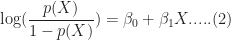
As mentioned earlier, we are after the probability of class membership so we must ensure that the hypothesis function (a fancy word for the model) always lies between 0 and 1. The function assumed in logistic regression is:

You can verify that 


Figure 1: Logistic function
As an aside, you might be wondering where the name logistic comes from. An equivalent way of expressing the above equation is:
The quantity on the left is the logarithm of the odds. So, the model is a linear regression of the log-odds, sometimes called logit, and hence the name logistic.
The problem is to find the values of 

Where 
It should be noted that in practice one works with the log likelihood because it is easier to work with mathematically. Moreover, one minimises the negative log likelihood which, of course, is the same as maximising the log likelihood. The quantity one minimises is thus:
However, these are technical details that I mention only for completeness. As you will see next, they have little bearing on the practical use of logistic regression.
Logistic regression in R – an example
In this example, we’ll use the logistic regression option implemented within the glm function that comes with the base R installation. This function fits a class of models collectively known as generalized linear models. We’ll apply the function to the Pima Indian Diabetes dataset that comes with the mlbench package. The code is quite straightforward – particularly if you’ve read earlier articles in my “gentle introduction” series – so I’ll just list the code below noting that the logistic regression option is invoked by setting family=”binomial” in the glm function call.
Here we go:
Although this seems pretty good, we aren’t quite done because there is an issue that is lurking under the hood. To see this, let’s examine the information output from the model summary, in particular the coefficient estimates (i.e. estimates for 
- Column 2 in the table lists coefficient estimates.
- Column 3 list s the standard error of the estimates (the larger the standard error, the less confident we are about the estimate)
- Column 4 the z statistic (which is the coefficient estimate (column 2) divided by the standard error of the estimate (column 3)) and
- The last column (Pr(>|z|) lists the p-value, which is the probability of getting the listed estimate assuming the predictor has no effect. In essence, the smaller the p-value, the more significant the estimate is likely to be.
From the table we can conclude that only 4 predictors are significant – pregnant, glucose, mass and pedigree (and possibly a fifth – pressure). The other variables have little predictive power and worse, may contribute to overfitting. They should, therefore, be eliminated and we’ll do that in a minute. However, there’s an important point to note before we do so…
In this case we have only 9 variables, so are able to identify the significant ones by a manual inspection of p-values. As you can well imagine, such a process will quickly become tedious as the number of predictors increases. Wouldn’t it be be nice if there were an algorithm that could somehow automatically shrink the coefficients of these variables or (better!) set them to zero altogether? It turns out that this is precisely what lasso and its close cousin, ridge regression, do.
Ridge and Lasso
Recall that the values of the logistic regression coefficients 


and

Where 
In the case of ridge regression, the effect of the penalty term is to shrink the coefficients that contribute most to the error. Put another way, it reduces the magnitude of the coefficients that contribute to increasing 
Let’s illustrate this through an example. We’ll use the glmnet package which implements a combined version of ridge and lasso (called elastic net). Instead of minimising (4) or (5) above, glmnet minimises:
![L +\lambda[ (1-\alpha)\sum [\beta_1^2 + \alpha\sum|\beta_1|]....(6)](https://s0.wp.com/latex.php?latex=L+%2B%5Clambda%5B+%281-%5Calpha%29%5Csum+%5B%5Cbeta_1%5E2+%2B+%5Calpha%5Csum%7C%5Cbeta_1%7C%5D....%286%29&bg=ffffff&fg=1c1c1c&s=0&c=20201002)
where 


Lasso regularisation using glmnet
Let’s reanalyse the Pima Indian Diabetes dataset using glmnet with
- does not have a formula interface, so one has to input the predictors as a matrix and the class labels as a vector.
- does not accept categorical predictors, so one has to convert these to numeric values before passing them to glmnet.
The glmnet function model.matrix creates the matrix and also converts categorical predictors to appropriate dummy variables.
Another important point to note is that we’ll use the function cv.glmnet, which automatically performs a grid search to find the optimal value of
OK, enough said, here we go:
The plot is shown in Figure 2 below:
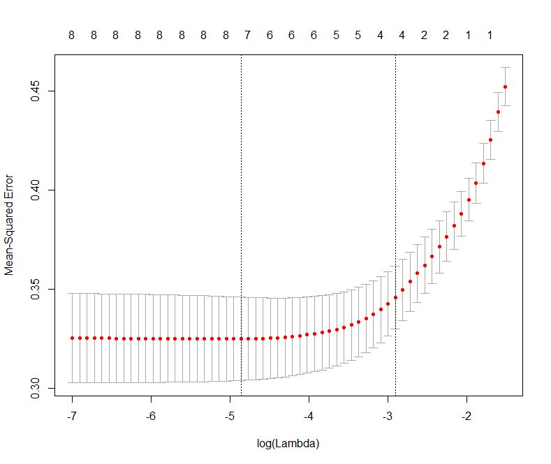
Figure 2: Error as a function of lambda (select lambda that minimises error)
The plot shows that the log of the optimal value of lambda (i.e. the one that minimises the root mean square error) is approximately -5. The exact value can be viewed by examining the variable lambda_min in the code below. In general though, the objective of regularisation is to balance accuracy and simplicity. In the present context, this means a model with the smallest number of coefficients that also gives a good accuracy. To this end, the cv.glmnet function finds the value of lambda that gives the simplest model but also lies within one standard error of the optimal value of lambda. This value of lambda (lambda.1se) is what we’ll use in the rest of the computation. Interested readers should have a look at this article for more on lambda.1se vs lambda.min.
The output shows that only those variables that we had determined to be significant on the basis of p-values have non-zero coefficients. The coefficients of all other variables have been set to zero by the algorithm! Lasso has reduced the complexity of the fitting function massively…and you are no doubt wondering what effect this has on accuracy. Let’s see by running the model against our test data:
Which is a bit less than what we got with the more complex model. So, we get a similar out-of-sample accuracy as we did before, and we do so using a way simpler function (4 non-zero coefficients) than the original one (9 nonzero coefficients). What this means is that the simpler function does at least as good a job fitting the signal in the data as the more complicated one. The bias-variance tradeoff tells us that the simpler function should be preferred because it is less likely to overfit the training data.
Paraphrasing William of Ockham: all other things being equal, a simple hypothesis should be preferred over a complex one.
Wrapping up
In this post I have tried to provide a detailed introduction to logistic regression, one of the simplest (and oldest) classification techniques in the machine learning practitioners arsenal. Despite it’s simplicity (or I should say, because of it!) logistic regression works well for many business applications which often have a simple decision boundary. Moreover, because of its simplicity it is less prone to overfitting than flexible methods such as decision trees. Further, as we have shown, variables that contribute to overfitting can be eliminated using lasso (or ridge) regularisation, without compromising out-of-sample accuracy. Given these advantages and its inherent simplicity, it isn’t surprising that logistic regression remains a workhorse for data scientists.
The improbability of success
Anyone who has tidied up after a toddler intuitively understands that making a mess is far easier than creating order. The fundamental reason for this is that the number of messy states in the universe (or a toddler’s room) far outnumbers the ordered ones. As this point might not be obvious, I’ll demonstrate it via a simple thought experiment involving marbles:
Throw three marbles onto a flat surface. When the marbles come to rest, you are most likely to end up with a random configuration as in Figure 1.

Figure 1: A random configuration of 3 marbles
Indeed, you’d be extremely surprised if the three ended up being collinear as in Figure 2. Note that Figure 2 is just one example of many collinear possibilities, but the point I’m making is that if the marbles are thrown randomly, they are more likely to end up in a random state than a lined-up one.

Figure 2: an unlikely (ordered) configuration
This raises a couple of questions:
Question: On what basis can one claim that the collinear configuration is tidier or more ordered than the non-collinear one?
Naive answer: It looks more ordered. Yes, tidiness is in the eye of the beholder so it is necessarily subjective. However, I’ll wager that if one took a poll, an overwhelming number of people would say that the configuration in Figure 2 is more ordered than the one in Figure 1.
More sophisticated answer : The “state” of collinear marbles can be described using 2 parameters, the slope and intercept of the straight line that three marbles lie on (in any coordinate system) whereas the description of the nonlinear state requires 3 parameters. The first state is tidier because it requires fewer parameters. Another way to think about is that the line can be described by two marbles; the third one is redundant as far as the description of the state is concerned.
Question: Why is a tidier configuration less likely than a messy one?
Answer: May be you see this intuitively and need no proof, but here’s one just in case. Imagine rolling the three marbles one after the other. The first two, regardless of where they end up, will necessarily lie along a line (two points lie on the straight line joining them). Now, I think it is easy to see that if we throw the third marble randomly, it is highly unlikely end up on that line. Indeed, for the third marble to end up exactly on the same straight line requires a coincidence of near cosmic proportions.
I know, I know, this is not a proof, but I trust it makes the point.
Now, although it is near impossible to get to a collinear end state via random throws, it is possible to approximate it by changing the way we throw the marbles. Here’s how:
- Throw the marbles consecutively rather than in one go.
- When throwing the third marble, adjust its initial speed and direction in a way that takes into account the positions of the two marbles that are already on the surface. Remember these two already define a straight line.
The third throw is no longer random because it is designed to maximise the chance that the last marble will get as close as possible to the straight line defined by the first two. Done right, you’ll end up with something closer to the configuration in Figure 3 rather than the one in Figure 2.

Figure 3: an “approximately ordered” state
Now you’re probably wondering what this has to do with success. I’ll make the connection via an example that will be familiar to many readers of this blog: an organisation’s strategy. However, as I will reiterate later, the arguments I present are very general and can be applied to just about any initiative or situation.
Typically, a strategy sets out goals for an organisation and a plan to achieve them in a specified timeframe. The goals define a number of desirable outcomes, or states which, by design, are constrained to belong to a (very) small subset of all possible states the organisation can end up in. In direct analogy with the simple model discussed above it is clear that, left to its own devices, the organisation is more likely to end up in one of the much overwhelmingly larger number of “failed states” than one of the successful ones. Notwithstanding the popular quote about there being many roads to success, in reality there are a great many more roads to failure.
Of course, that’s precisely why organisations are never “left to their own devices.” Indeed, a strategic plan specifies actions that are intended to make a successful state more likely than an unsuccessful one. However, no plan can guarantee success; it can, at best, make it more likely. As in the marble game, success is ultimately a matter of chance, even when we take actions to make it more likely.
If we accept this, the key question becomes: how can one design a strategy that improves the odds of success? The marble analogy suggests a way to do this is to:
- Define success in terms of an end state that is a natural extension of your current state.
- Devise a plan to (approximately) achieve that end state. Such a plan will necessarily build on the current state rather than change it wholesale. Successful change is an evolutionary process rather than a revolutionary one.
My contention is that these points are often ignored by management strategists. More often than not, they will define an end state based on a textbook idealisation, consulting model or (horror!) best practice. The marble analogy shows why copying others is unlikely to succeed.
Figure 4 shows a variant of the marble game in which we have two sets of marbles (or organisations!), one blue, as before, and the other red.

Figure 4: Two distinct configurations of marbles (or organisations)
Now, it is considerably harder to align an additional marble with both sets of marbles than the blue one alone. Here’s why…
To align with both sets, the new marble has to end up close to the point that lies at the intersection of the blue and red lines in Figure 5. In contrast, to align with the blue set alone, all that’s needed is for it to get close to any point on the blue line.
QED!

Figure 5: Why copying others is not a good idea (see text for explanation)
Finally, on a broader note, it should be clear that the arguments made above go beyond organisational strategies. They apply to pretty much any planned action, whether at work or in one’s personal life.
So, to sum up: when developing an organisational (or personal) strategy, the first step is to understand where you are and then identify the minimal actions you need to take in order to get to an “improved” state that is consistent with your current one. Yes, this is akin to the incremental and evolutionary approach that Agilistas and Leaners have been banging on about for years. However, their prescriptions focus on specific areas: software development and process improvement. My point is that the basic principles are way broader because they are a direct consequence of a fundamental fact regarding the relative likelihood of order and disorder in a toddler’s room, an organisation, or even the universe at large.
Uncertainty, ambiguity and the art of decision making
A common myth about decision making in organisations is that it is, by and large, a rational process. The term rational refers to decision-making methods that are based on the following broad steps:
- Identify available options.
- Develop criteria for rating options.
- Rate options according to criteria developed.
- Select the top-ranked option.
Although this appears to be a logical way to proceed it is often difficult to put into practice, primarily because of uncertainty about matters relating to the decision.
Uncertainty can manifest itself in a variety of ways: one could be uncertain about facts, the available options, decision criteria or even one’s own preferences for options.
In this post, I discuss the role of uncertainty in decision making and, more importantly, how one can make well-informed decisions in such situations.
A bit about uncertainty
It is ironic that the term uncertainty is itself vague when used in the context of decision making. There are at least five distinct senses in which it is used:
- Uncertainty about decision options.
- Uncertainty about one’s preferences for options.
- Uncertainty about what criteria are relevant to evaluating the options.
- Uncertainty about what data is needed (data relevance).
- Uncertainty about the data itself (data accuracy).
Each of these is qualitatively different: uncertainty about data accuracy (item 5 above) is very different from uncertainty regarding decision options (item 1). The former can potentially be dealt with using statistics whereas the latter entails learning more about the decision problem and its context, ideally from different perspectives. Put another way, the item 5 is essentially a technical matter whereas item 1 is a deeper issue that may have social, political and – as we shall see – even behavioural dimensions. It is therefore reasonable to expect that the two situations call for vastly different approaches.
Quantifiable uncertainty
A common problem in project management is the estimation of task durations. In this case, what’s requested is a “best guess” time (in hours or days) it will take to complete a task. Many project schedules represent task durations by point estimates, i.e. by single numbers. The Gantt Chart shown in Figure 1 is a common example. In it, each task duration is represented by its expected duration. This is misleading because the single number conveys a sense of certainty that is unwarranted. It is far more accurate, not to mention safer, to quote a range of possible durations.

Figure 1: Gantt Chart (courtesy Wikimedia)
In general, quantifiable uncertainties, such as those conveyed in estimates, should always be quoted as ranges – something along the following lines: task A may take anywhere between 2 and 8 days, with a most likely completion time of 4 days (Figure 2).

Figure 2: Task completion likelihood (3 point estimates)
In this example, aside from stating that the task will finish sometime between 2 and 4 days, the estimator implicitly asserts that the likelihood of finishing before 2 days or after 8 days is zero. Moreover, she also implies that some completion times are more likely than others. Although it may be difficult to quantify the likelihood exactly, one can begin by making simple (linear!) approximations as shown in Figure 3.
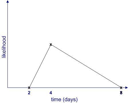
Figure 3: Simple probability distribution based on the estimates in Fig 2
The key takeaway from the above is that quantifiable uncertainties are shapes rather than single numbers. See this post and this one for details for how far this kind of reasoning can take you. That said, one should always be aware of the assumptions underlying the approximations. Failure to do so can be hazardous to the credibility of estimators!
Although I haven’t explicitly said so, estimation as described above has a subjective element. Among other things, the quality of an estimate depends on the judgement and experience of the estimator. As such, it is prone to being affected by errors of judgement and cognitive biases. However, provided one keeps those caveats in mind, the probability-based approach described above is suited to situations in which uncertainties are quantifiable, at least in principle. That said, let’s move on to more complex situations in which uncertainties defy quantification.
Introducing ambiguity
The economist Frank Knight was possibly the first person to draw the distinction between quantifiable and unquantifiable uncertainties. To make things really confusing, he called the former risk and the latter uncertainty. In his doctoral thesis, published in 1921, wrote:
…it will appear that a measurable uncertainty, or “risk” proper, as we shall call the term, is so far different from an unmeasurable one that it is not in effect an uncertainty at all. We shall accordingly restrict the term “uncertainty” to cases of the non-quantitative type (p.20)
Terminology has moved on since Knight’s time, the term uncertainty means lots of different things, depending on context. In this piece, we’ll use the term uncertainty to refer to quantifiable uncertainty (as in the task estimate of the previous section) and use ambiguity to refer to non–quantifiable uncertainty. In essence, then, we’ll use the term uncertainty for situations where we know what we’re measuring (i.e. the facts) but are uncertain about its numerical or categorical values whereas we’ll use the word ambiguity to refer to situations in which we are uncertain about what the facts are or which facts are relevant.
As a test of understanding, you may want to classify each of the five points made in the second section of this post as either uncertain or ambiguous (Answers below)
Answer: 1 through 4 are ambiguous and 5 is uncertain.
How ambiguity manifests itself in decision problems
The distinction between uncertainty and ambiguity points to a problem with quantitative decision-making techniques such as cost-benefit analysis, multicriteria decision making methods or analytic hierarchy process. All these methods assume that decision makers are aware of all the available options, their preferences for them, the relevant evaluation criteria and the data needed. This is almost never the case for consequential decisions. To see why, let’s take a closer look at the different ways in which ambiguity can play out in the rational decision making process mentioned at the start of this article.
- The first step in the process is to identify available options. In the real world, however, options often cannot be enumerated or articulated fully. Furthermore, as options are articulated and explored, new options and sub-options tend to emerge. This is particularly true if the options depend on how future events unfold.
- The second step is to develop criteria for rating options. As anyone who has been involved in deciding on a contentious issue will confirm, it is extremely difficult to agree on a set of decision criteria for issues that affect different stakeholders in different ways. Building a new road might improve commute times for one set of stakeholders but result in increased traffic in a residential area for others. The two criteria will be seen very differently by the two groups. In this case, it is very difficult for the two groups to agree on the relative importance of the criteria or even their legitimacy. Indeed, what constitutes a legitimate criterion is a matter of opinion.
- The third step is to rate options. The problem here is that real-world options often cannot be quantified or rated in a meaningful way. Many of life’s dilemmas fall into this category. For example, a decision to accept or decline a job offer is rarely made on the basis of material gain alone. Moreover, even where ratings are possible, they can be highly subjective. For example, when considering a job offer, one candidate may give more importance to financial matters whereas another might consider lifestyle-related matters (flexi-hours, commuting distance etc.) to be paramount. Another complication here is that there may not be enough information to settle the matter conclusively. As an example, investment decisions are often made on the basis of quantitative information that is based on questionable assumptions.
A key consequence of the above is that such ambiguous decision problems are socially complex – i.e. different stakeholders could have wildly different perspectives on the problem itself. One could say the ambiguity experienced by an individual is compounded by the group.
Before going on I should point out that acute versions of such ambiguous decision problems go by many different names in the management literature. For example:
- Horst Rittel called them wicked problems..
- Russell Ackoff referred to them as messes.
- Herbert Simon labelled them non-programmable problems.
All these terms are more or less synonymous: the root cause of the difficulty in every case is ambiguity (or unquantifiable uncertainty), which prevents a clear formulation of the problem.
Social complexity is hard enough to tackle as it is, but there’s another issue that makes things even harder: ambiguity invariably triggers negative emotions such as fear and anxiety in individuals who make up the group. Studies in neuroscience have shown that in contrast to uncertainty, which evokes logical responses in people, ambiguity tends to stir up negative emotions while simultaneously suppressing the ability to think logically. One can see this playing out in a group that is debating a contentious decision: stakeholders tend to get worked up over issues that touch on their values and identities, and this seems to limit their ability to look at the situation objectively.
Tackling ambiguity
Summarising the discussion thus far: rational decision making approaches are based on the assumption that stakeholders have a shared understanding of the decision problem as well as the facts and assumptions around it. These conditions are clearly violated in the case of ambiguous decision problems. Therefore, when confronted with a decision problem that has even a hint of ambiguity, the first order of the day is to help the group reach a shared understanding of the problem. This is essentially an exercise in sensemaking, the art of collaborative problem formulation. However, this is far from straightforward because ambiguity tends to evoke negative emotions and attendant defensive behaviours.
The upshot of all this is that any approach to tackle ambiguity must begin by taking the concerns of individual stakeholders seriously. Unless this is done, it will be impossible for the group to coalesce around a consensus decision. Indeed, ambiguity-laden decisions in organisations invariably fail when they overlook concerns of specific stakeholder groups. The high failure rate of organisational change initiatives (60-70% according to this Deloitte report) is largely attributable to this point
There are a number of techniques that one can use to gather and synthesise diverse stakeholder viewpoints and thus reach a shared understanding of a complex or ambiguous problem. These techniques are often referred to as problem structuring methods (PSMs). I won’t go into these in detail here; for an example check out Paul Culmsee’s articles on dialogue mapping and Barry Johnson’s introduction to polarity management. There are many more techniques in the PSM stable. All of them are intended to help a group reconcile different viewpoints and thus reach a common basis from which one can proceed to the next step (i.e., make a decision on what should be done). In other words, these techniques help reduce ambiguity.
But there’s more to it than a bunch of techniques. The main challenge is to create a holding environment that enables such techniques to work. I am sure readers have been involved in a meeting or situation where the outcome seems predetermined by management or has been undermined by self- interest. When stakeholders sense this, no amount of problem structuring is going to help. In such situations one needs to first create the conditions for open dialogue to occur. This is precisely what a holding environment provides.
Creating such a holding environment is difficult in today’s corporate world, but not impossible. Note that this is not an idealist’s call for an organisational utopia. Rather, it involves the application of a practical set of tools that address the diverse, emotion-laden reactions that people often have when confronted with ambiguity. It would take me too far afield to discuss PSMs and holding environments any further here. To find out more, check out my papers on holding environments and dialogue mapping in enterprise IT projects, and (for a lot more) the Heretic’s Guides that I co-wrote with Paul Culmsee.
The point is simply this: in an ambiguous situation, a good decision – whatever it might be – is most likely to be reached by a consultative process that synthesises diverse viewpoints rather than by an individual or a clique. However, genuine participation (the hallmark of a holding environment) in such a process will occur only after participants’ fears have been addressed.
Wrapping up
Standard approaches to decision making exhort managers and executives to begin with facts, and if none are available, to gather them diligently prior to making a decision. However, most real-life decisions are fraught with uncertainty so it may be best to begin with what one doesn’t know, and figure out how to make the possible decision under those “constraints of ignorance.” In this post I’ve attempted to outline what such an approach would entail. The key point is to figure out the kind uncertainty one is dealing with and choosing an approach that works for it. I’d argue that most decision making debacles stem from a failure to appreciate this point.
Of course, there’s a lot more to this approach than I can cover in the span of a post, but that’s a story for another time.
Note: This post is written as an introduction to the Data and Decision Making subject that is part of the core curriculum of the Master of Data Science and Innovation program at UTS. I’m co-teaching the subject in Autumn 2018 with Rory Angus and Alex Scriven.


