Eight to Late

Introduction

Welcome to the second part of my introductory series on text analysis using R (the first article can be accessed here).  My aim in the present piece is to provide a  practical introduction to cluster analysis. I’ll begin with some background before moving on to the nuts and bolts of clustering. We have a fair bit to cover, so let’s get right to it.

A common problem when analysing large collections of documents is to categorize them in some meaningful way. This is easy enough if one has a predefined classification scheme that is known to fit the collection (and if the collection is small enough to be browsed manually). One can then simply scan the documents, looking for keywords appropriate to each category and classify the documents based on the results. More often than not, however, such a classification scheme is not available and the collection too large. One then needs to use algorithms that can classify documents automatically based on their structure and content.

The present post is a practical introduction to a couple of automatic text categorization techniques, often referred to as clustering algorithms.  As the Wikipedia article on clustering tells us:

Cluster analysis or clustering is the task of grouping a set of objects in such a way that objects in the same group (called a cluster) are more similar (in some sense or another) to each other than to those in other groups (clusters).

As one might guess from the above, the results of clustering depend rather critically on the method one uses to group objects. Again, quoting from the Wikipedia piece:

Cluster analysis itself is not one specific algorithm, but the general task to be solved. It can be achieved by various algorithms that differ significantly in their notion of what constitutes a cluster and how to efficiently find them. Popular notions of clusters include groups with small distances [Note: we’ll use distance-based methods] among the cluster members, dense areas of the data space, intervals or particular statistical distributions [i.e. distributions of words within documents and the entire collection].

…and a bit later:

…the notion of a “cluster” cannot be precisely defined, which is one of the reasons why there are so many clustering algorithms. There is a common denominator: a group of data objects. However, different researchers employ different cluster models, and for each of these cluster models again different algorithms can be given. The notion of a cluster, as found by different algorithms, varies significantly in its properties. Understanding these “cluster models” is key to understanding the differences between the various algorithms.

An upshot of the above is that it is not always straightforward to interpret the output of clustering algorithms. Indeed, we will see this in the example discussed below.

With that said for an introduction, let’s move on to the nut and bolts of clustering.

Preprocessing the corpus

In this section I cover the steps required to create the R objects necessary in order to do clustering. It goes over territory that I’ve covered in detail in the first article in this series – albeit with a few tweaks, so you may want to skim through even if you’ve read my previous piece.

To begin with I’ll assume you have R and RStudio (a free development environment for R) installed on your computer and are familiar with the basic functionality in the text mining ™ package.  If you need help with this, please look at the instructions in my previous article on text mining.

As in the first part of this series,  I will use 30 posts from my blog as the example collection (or corpus, in text mining-speak). The corpus can be downloaded here. For completeness, I will run through the entire sequence of steps – right from loading the corpus into R, to running the two clustering algorithms.

Ready? Let’s go…

The first step is to fire up RStudio and navigate to the directory in which you have unpacked the example corpus. Once this is done, load the text mining package, tm.  Here’s the relevant code (Note: a complete listing of the code in this article can be accessed here):

Note: R commands are in blue, output in black or red; lines that start with # are comments.

If you get an error here, you probably need to download and install the tm package. You can do this in RStudio by going to Tools > Install Packages and entering “tm”. When installing a new package, R automatically checks for and installs any dependent packages.

The next step is to load the collection of documents into an object that can be manipulated by functions in the tm package.

The next step is to clean up the corpus. This includes things such as transforming to a consistent case, removing non-standard symbols & punctuation, and removing numbers (assuming that numbers do not contain useful information, which is the case here):

Note: please see my previous article for more on content_transformer and the toSpace function defined above.

Next we remove stopwords – common words (like “a” “and” “the”, for example) and eliminate extraneous whitespaces.

At this point it is critical to inspect the corpus because  stopword removal in tm can be flaky. Yes, this is annoying but not a showstopper because one can remove problematic words manually once one has identified them – more about this in a minute.

Next, we stem the document – i.e. truncate words to their base form. For example, “education”, “educate” and “educative” are stemmed to “educat.”:

Stemming works well enough, but there are some fixes that need to be done due to my inconsistent use of British/Aussie and US English. Also, we’ll take this opportunity to fix up some concatenations like “andgovernance” (see paragraph printed out above). Here’s the code:

The next step is to remove the stopwords that were missed by R. The best way to do this  for a small corpus is to go through it and compile a list of words to be eliminated. One can then create a custom vector containing words to be removed and use the removeWords transformation to do the needful. Here is the code (Note:  + indicates a continuation of a statement from the previous line):

Again, it is a good idea to check that the offending words have really been eliminated.

The final preprocessing step is to create a document-term matrix (DTM) – a matrix that lists all occurrences of words in the corpus.  In a DTM, documents are represented by rows and the terms (or words) by columns.  If a word occurs in a particular document n times, then the matrix entry for corresponding to that row and column is n, if it doesn’t occur at all, the entry is 0.

Creating a DTM is straightforward– one simply uses the built-in DocumentTermMatrix function provided by the tm package like so:

This brings us to the end of the preprocessing phase. Next, I’ll briefly explain how distance-based algorithms work before going on to the actual work of clustering.

An intuitive introduction to the algorithms

As mentioned in the introduction, the basic idea behind document or text clustering is to categorise documents into groups based on likeness. Let’s take a brief look at how the algorithms work their magic.

Consider the structure of the DTM. Very briefly, it is a matrix in which the documents are represented as rows and words as columns. In our case, the corpus has 30 documents and 4131 words, so the DTM is a 30 x 4131 matrix.  Mathematically, one can think of this matrix as describing a 4131 dimensional space in which each of the words represents a coordinate axis and each document is represented as a point in this space. This is hard to visualise of course, so it may help to illustrate this via a two-document corpus with only three words in total.

Consider the following corpus:

Document A: “five plus five”

Document B: “five plus six”

These two  documents can be represented as points in a 3 dimensional space that has the words “five” “plus” and “six” as the three coordinate axes (see figure 1).

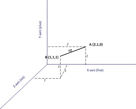
Figure 1: Documents A and B as points in a 3-word space

Now, if each of the documents can be thought of as a point in a space, it is easy enough to take the next logical step which is to define the notion of a distance between two points (i.e. two documents). In figure 1 the distance between A and B  (which I denote as )is the length of the line connecting the two points, which is simply, the sum of the squares of the differences between the coordinates of the two points representing the documents.

Generalising the above to the 4131 dimensional space at hand, the distance between two documents (let’s call them X and Y) have coordinates (word frequencies) 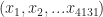  and , then one can define the straight line distance (also called Euclidean distance)   between them as:

It should be noted that the Euclidean distance that I have described is above is not the only possible way to define distance mathematically. There are many others but it would take me too far afield to discuss them here – see this article for more  (and don’t be put off by the term metric,  a metric  in this context is merely a distance)

What’s important here is the idea that one can define a numerical distance between documents. Once this is grasped, it is easy to understand the basic idea behind how (some) clustering algorithms work – they group documents based on distance-related criteria.  To be sure, this explanation is simplistic and glosses over some of the complicated details in the algorithms. Nevertheless it is a reasonable, approximate explanation for what goes on under the hood. I hope purists reading this will agree!

Finally, for completeness I should mention that there are many clustering algorithms out there, and not all of them are distance-based.

Hierarchical clustering

The first algorithm we’ll look at is hierarchical clustering. As the Wikipedia article on the topic tells us, strategies for hierarchical clustering fall into two types:

Agglomerative: where we start out with each document in its own cluster. The algorithm  iteratively merges documents or clusters that are closest to each other until the entire corpus forms a single cluster. Each merge happens at a different (increasing) distance.

Divisive:  where we start out with the entire set of documents in a single cluster. At each step  the algorithm splits the cluster recursively until each document is in its own cluster. This is basically the inverse of an agglomerative strategy.

The algorithm we’ll use is hclust which does agglomerative hierarchical clustering. Here’s a simplified description of how it works:

1. Assign each document to its own (single member) cluster
2. Find the pair of clusters that are closest to each other and merge them. So you now have one cluster less than before.
3. Compute distances between the new cluster and each of the old clusters.
4. Repeat steps 2 and 3 until you have a single cluster containing all documents.

We’ll need to do a few things before running the algorithm. Firstly, we need to convert the DTM into a standard matrix which can be used by dist, the distance computation function in R (the DTM is not stored as a standard matrix). We’ll also shorten the document names so that they display nicely in the graph that we will use to display results of hclust (the names I have given the documents are just way too long). Here’s the relevant code:

Next we run hclust. The algorithm offers several options check out the documentation for details. I use a popular option called Ward’s method – there are others, and I suggest you experiment with them  as each of them gives slightly different results making interpretation somewhat tricky (did I mention that clustering is as much an art as a science??). Finally, we visualise the results in a dendogram (see Figure 2 below).

Figure 2: Dendogram from hierarchical clustering of corpus

A few words on interpreting dendrograms for hierarchical clusters: as you work your way down the tree in figure 2, each branch point you encounter is the distance at which a cluster merge occurred. Clearly, the most well-defined clusters are those that have the largest separation; many closely spaced branch points indicate a lack of dissimilarity (i.e. distance, in this case) between clusters. Based on this, the figure reveals that there are 2 well-defined clusters – the first one consisting of the three documents at the right end of the cluster and the second containing all other documents. We can display the clusters on the graph using the rect.hclust function like so:

The result is shown in the figure below.

Figure 3: 2 cluster grouping

The figures 4 and 5 below show the grouping for 3,  and 5 clusters.

Figure 4: 3 cluster grouping

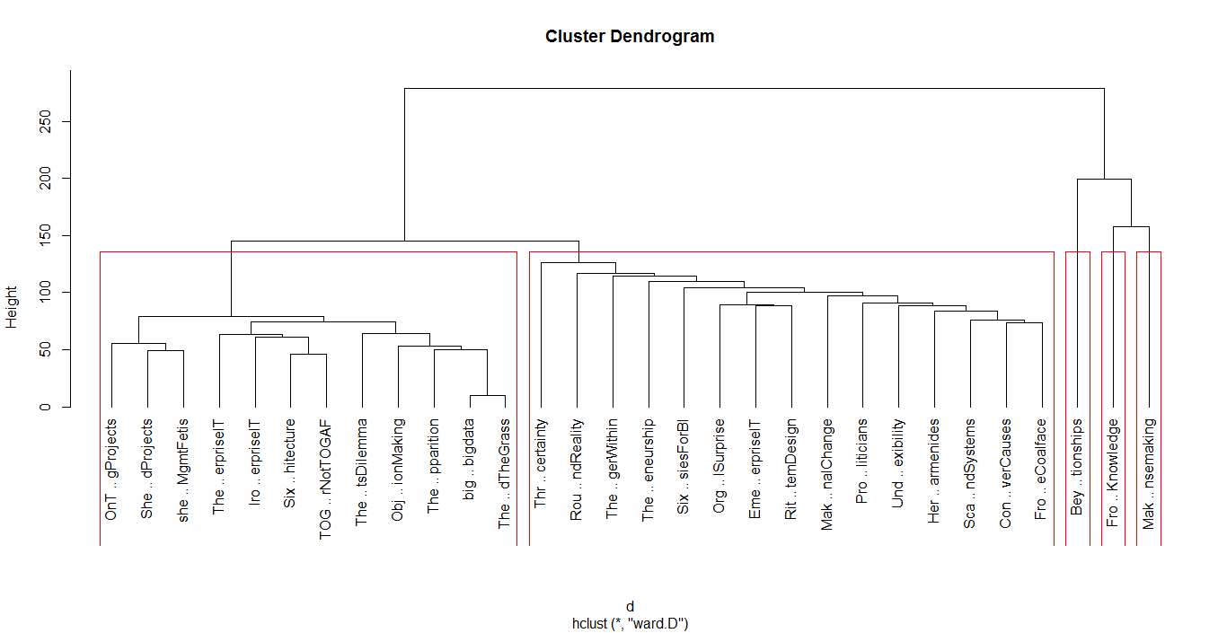
Figure 5: 5 cluster grouping

I’ll make just one point here: the 2 cluster grouping seems the most robust one as it happens at large distance, and is cleanly separated (distance-wise) from the 3 and 5 cluster grouping. That said, I’ll leave you to explore the ins and outs of hclust on your own and move on to our next algorithm.

K means clustering

In hierarchical clustering we did not specify the number of clusters upfront. These were determined by looking at the dendogram after the algorithm had done its work.  In contrast, our next algorithm – K means –   requires us to define the number of clusters upfront (this number being the “k” in the name). The algorithm then generates k document clusters in a way that ensures the within-cluster distances from each cluster member to the centroid (or geometric mean) of the cluster is minimised.

Here’s a simplified description of the algorithm:

1. Assign the documents randomly to k bins
2. Compute the location of the centroid of each bin.
3. Compute the distance between each document and each centroid
4. Assign each document to the bin corresponding to the centroid closest to it.
5. Stop if no document is moved to a new bin, else go to step 2.

An important limitation of the k means method is that the solution found by the algorithm corresponds to a local rather than global minimum (this figure from Wikipedia explains the difference between the two in a nice succinct way). As a consequence it is important to run the algorithm a number of times (each time with a different starting configuration) and then select the result that gives the overall lowest sum of within-cluster distances for all documents.  A simple check that a solution is robust is to run the algorithm for an increasing number of initial configurations until the result does not change significantly. That said, this procedure does not guarantee a globally optimal solution.

I reckon that’s enough said about the algorithm, let’s get on with it using it. The relevant function, as you might well have guessed is kmeans. As always, I urge you to check the documentation to understand the available options. We’ll use the default options for all parameters excepting nstart which we set to 100. We also plot the result using the clusplot function from the cluster library (which you may need to install. Reminder you can install packages via the Tools>Install Packages menu in RStudio)

The plot is shown in Figure 6.

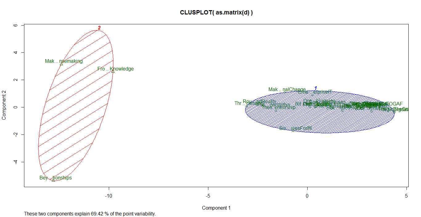
Figure 6: principal component plot (k=2)

The cluster plot shown in the figure above needs a bit of explanation. As mentioned earlier, the clustering algorithms work in a mathematical space whose dimensionality equals the number of words in the corpus (4131 in our case). Clearly, this is impossible to visualize.  To handle this, mathematicians have invented a dimensionality reduction technique called Principal Component Analysis which reduces the number of dimensions to 2 (in this case) in such a way that the reduced dimensions capture as much of the variability between the clusters as possible (and hence the comment, “these two components explain 69.42% of the point variability” at the bottom of the plot in figure 6)

(Aside  Yes I realize the figures are hard to read because of the overly long names, I leave it to you to fix that. No excuses, you know how…:-))

Running the algorithm and plotting the results for k=3 and 5 yields the figures below.

Figure 7: Principal component plot (k=3)

Figure 8: Principal component plot (k=5)

Choosing k

Recall that the k means algorithm requires us to specify k upfront. A natural question then is: what is the best choice of k? In truth there is no one-size-fits-all answer to this question, but there are some heuristics that might sometimes help guide the choice. For completeness I’ll describe one below even though it is not much help in our clustering problem.

In my simplified description of the k means algorithm I mentioned that the technique attempts to minimise the sum of the distances between the points in a cluster and the cluster’s centroid. Actually, the quantity that is minimised is the total of the within-cluster sum of squares (WSS) between each point and the mean. Intuitively one might expect this quantity to be maximum when k=1 and then decrease as k increases, sharply at first and then less sharply as k reaches its optimal value.

The problem with this reasoning is that it often happens that the within cluster sum of squares never shows a slowing down in decrease of the summed WSS. Unfortunately this is exactly what happens in the case at hand.

I reckon a picture might help make the above clearer. Below is the R code to draw a plot of summed WSS as a function of k for k=2 all the way to 29 (1-total number of documents):

…and the figure below shows the resulting plot.

Figure 10: WSS as a function of k (“elbow plot”)

The plot clearly shows that there is no k for which the summed WSS flattens out (no distinct “elbow”).  As a result this method does not help. Fortunately, in this case  one can get a sensible answer using common sense rather than computation:  a choice of 2 clusters seems optimal because both algorithms yield exactly the same clusters and show the clearest cluster separation at this point (review the dendogram and cluster plots for k=2).

The meaning of it all

Now I must acknowledge an elephant in the room that I have steadfastly ignored thus far. The odds are good that you’ve seen it already….

It is this: what topics or themes do the (two) clusters correspond to?

Unfortunately this question does not have a straightforward answer. Although the algorithms suggest a 2-cluster grouping, they are silent on the topics or themes related to these.   Moreover,  as you will see if you experiment, the results of clustering depend on:

• The criteria for the construction of the DTM  (see the documentation for DocumentTermMatrix for options).
• The clustering algorithm itself.

Indeed, insofar as clustering is concerned, subject matter and corpus knowledge is the best way to figure out cluster themes. This serves to reinforce (yet again!) that clustering is as much an art as it is a science.

In the case at hand, article length seems to be an important differentiator between the 2 clusters found by both algorithms. The three articles in the smaller cluster are in the top 4 longest pieces in the corpus.  Additionally, the three pieces are related to sensemaking and dialogue mapping. There are probably other factors as well, but none that stand out as being significant. I should mention, however, that the fact that article length seems to play a significant role here suggests that it may be worth checking out the effect of scaling distances by word counts or using other measures such a cosine similarity – but that’s a topic for another post! (Note added on Dec 3 2015: check out my article on visualizing relationships between documents using network graphs for a detailed discussion on cosine similarity)

The take home lesson is that  is that the results of clustering are often hard to interpret. This should not be surprising – the algorithms cannot interpret meaning, they simply chug through a mathematical optimisation problem. The onus is on the analyst to figure out what it means…or if it means anything at all.

Conclusion

This brings us to the end of a long ramble through clustering.  We’ve explored the two most common methods:  hierarchical and k means clustering (there are many others available in R, and I urge you to explore them). Apart from providing the detailed steps to do clustering, I have attempted to provide an intuitive explanation of how the algorithms work.  I hope I have succeeded in doing so. As always your feedback would be very welcome.

Finally, I’d like to reiterate an important point:  the results of our clustering exercise do not have a straightforward interpretation, and this is often the case in cluster analysis. Fortunately I can close on an optimistic note. There are other text mining techniques that do a better job in grouping documents based on topics and themes rather than word frequencies alone.   I’ll discuss this in the next article in this series.  Until then, I wish you many enjoyable hours exploring the ins and outs of clustering.

Note added on September 29th 2015:

If you liked this article, you might want to check out its sequel – an introduction to topic modeling.