Eight to Late

Bayes Theorem for project managers

Introduction

Projects are fraught with uncertainty, so it is no surprise that the language and tools of probability are making their way into project management practice. A good example of this is the use of Monte Carlo methods to estimate project variables. Such tools enable the project manager to present estimates in terms of probabilities (e.g. there’s a 90% chance that a project will finish on time) rather than illusory certainties. Now, it often happens that we want to find the probability of an event occurring given that another event has occurred. For example, one might want to find the probability that a project will finish on time given that a major scope change has already occurred. Such conditional probabilities, as they are referred to in statistics, can be evaluated using Bayes Theorem. This post is a discussion of Bayes Theorem using an example from project management.

Bayes theorem by example

All project managers want to know whether the projects they’re working on will finish on time. So, as our example, we’ll assume that a project manager asks the question: what’s the probability that my project will finish on time? There are only two possibilties here: either the project finishes on (or before) time or it doesn’t. Let’s express this formally. Denoting the event the project finishes on (or before) time by $T$ , the event the project does not finish on (or before) time by $\tilde T$ and the probabilities of the two by $P(T)$ and $P(\tilde T)$ respectively, we have:

$P(T)+P(\tilde T) = 1$ ……(1),

Equation (1) is simply a statement of the fact that the sum of the probabilities of all possible outcomes must equal 1.

Fig 1. is a pictorial representation of the two events and how they relate to the entire universe of projects done by the organisation our project manager works in. The rectangular areas $A$ and $B$ represent the on time and not on time projects, and the sum of the two areas, $A+B$ , represents all projects that have been carried out by the organisation.

Fig 1: On Time and Not on Time projects

In terms of areas, the probabilities quoted above can be expressed as:

$P(T) = \displaystyle \frac{A}{A+B}$ ……(2),

and

$P(\tilde T) = \displaystyle \frac{B}{A+B}$ ……(3).

This also makes explicit the fact that the sum of the two probabilities must add up to one.

Now, there are several variables that can affect project completion time. Let’s look at just one of them: scope change. Let’s denote the event “there is a major change of scope” by $C$ and the complementary event (that there is no major change of scope) by $\tilde C$ .

Again, since the two possibilities cover the entire spectrum of outcomes, we have:

$P(C)+P(\tilde C) = 1$ ……(4).

Fig 2. is a pictorial representation of by $C$ and $\tilde C$ .

Fig 2: "Major Change" and "No Major Change" projects

The rectangular areas $D$ and $E$ represent the projects that have undergone major scope changes and those that haven’t respectively.

$P(C) = \displaystyle \frac{D}{D+E}$ ……(5),

and

$P(\tilde C) = \displaystyle \frac{E}{D+E}$ ……(6).

Clearly we also have $A+B=D+E$ since the number of projects completed is a fixed number, regardless of how it is arrived at.

Now things get interesting. One could ask the question: What is the probability of finishing on time given that there has been a major scope change? This is a conditional probability because it represents the likelihood that something will happen (on-time completion) on the condition that something else has already happened (scope change).

As a first step to answering the question posed in the previous paragraph, let’s combine the two events graphically. Fig 3 is a combination of Figs 1 and 2. It shows four possible events:

On Time with Major Change ( $T$ , $C$ ) – denoted by the rectangular area $AD$ in Fig 3.
On Time with No Major Change ( $T$ , $\tilde C$ ) – denoted by the rectangular area $AE$ in Fig 3.
Not On Time with Major Change ( $\tilde T$ , $C$ ) – denoted by the rectangular area $BD$ in Fig 3.
Not On Time with No Major Change ( $\tilde T$ , $\tilde latex C$) – denoted by the rectangular area $BE$ in Fig 3.

Fig 3: Combination of events shown in Figs 1 and 2

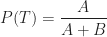
We’re interested in the probability that the project finishes on time given that it has suffered a major change in scope. In the notation of conditional probability, this is denoted by $P(T|C)$ . In terms of areas, this can be expressed as

$P(T|C) = \displaystyle \frac{AD}{AD+BD} = \frac{AD}{D}$ ……(7) ,

since $D$ (or equivalently $AD+BD$ ) represent all projects that have undergone a major scope change.

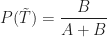
Similarly, the conditional probability that a project has undergone a major change given that it has come in on time, $P(C|T)$ , can be written as:

$P(C|T) =\displaystyle \frac{AD}{AD+AE} = \frac{AD}{A}$ ……(8) ,

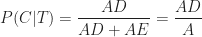
since $AD+AE=A$ .

Now, what I’m about to do next may seem like pointless algebraic jugglery, but bear with me…

Consider the ratio of the area $AD$ to the big outer rectangle (whose area is $A+B$ ) . This ratio can be expressed as follows:

$\displaystyle\frac{AD}{A+B}=\frac{AD}{D}\times\frac{D}{A+B}=\frac{AD}{A}\times\frac{A}{A+B}$ ……(9).

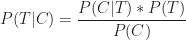
This is simply multiplying and dividing by the same factor ( $D$ in the second expression and $A$ in the third.

Written in the notation of conditional probabilities, the second and third expressions in (9) are:

$P(T|C)*P(C)=P(C|T)*P(T)$ ……(10),

which is Bayes theorem.

From the above discussion, it should be clear that Bayes theorem follows from the definition of conditional probability.

We can rewrite Bayes theorem in several equivalent ways:

$P(T|C)=\displaystyle\frac{P(C|T)*P(T)}{P(C)}$ ……(11),

$P(T|C)=\displaystyle\frac{P(C|T)P(T)}{ P(C|T)P(T)+P(C|\tilde T)P(\tilde T)}$ ……(12),

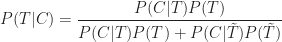
where the denominator in (12) follows from the fact that a project that undergoes a major change will either be on time or will not be on time (there is no other possibility).

A numerical example

To complete the discussion, let’s look at a numerical example.

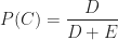
Assume our project manager has historical data on projects that have been carried out within the organisation. On analyzing the data, the PM finds that 60% of all projects finished on time. This implies:

$P(T) = 0.6$ ……(13),

and

$P(T) = 0.4$ ……(13),

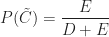
Let us assume that our organisation also tracks major changes made to projects in progress. Say 50% of all historical projects are found to have major changes. This implies:

$P(C) = 0.5$ ……(15).

Finally, let us assume that our project manager has access to detailed data on successful projects, and that an analysis of this data shows that 30% on time projects have undergone at least one major scope change. This gives:

$P(C|T) = 0.3$ ……(16).

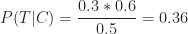
Equations (13) through (16) give us the numbers we need to calculated $P(T|C)$ using Bayes Theorem. Plugging the numbers in equation (11), we get:

$P(T|C)=\displaystyle\frac{0.3*0.6}{0.5}=0 .36$ ……(16)

So, in this organisation, if a project undergoes a major change then there’s a 36% probability that it will finish on time. Compare this to the 60% (unconditional) probability of finishing on time. Bayes theorem enables the project manager to quantify the impact of change in scope on project completion time, providing the relevant historical data is available. The italicised bit in the previous sentence is important; I’ll have more to say about it in the concluding section.

In closing this section I should emphasise that although my discussion of Bayes theorem is couched in terms of project completion times and scope changes, the arguments used are general. Bayes theorem holds for any pair of events.

Concluding remarks

It should be clear that the probability calculated in the previous section is an extrapolation based on past experience. In this sense, Bayes Theorem is a formal statement of the belief that one can predict the future based on past events. This goes beyond probability theory; it is an assumption that underlies much of science. It is important to emphasise that the prediction is based on enumeration, not analysis: it is solely based on ratios of the number of projects in one category versus the other; there is no attempt at finding a causal connection between the events of interest. In other words, Bayes theorem suggests there is a correlation between major changes in scope and delays, but it does not tell us why. The latter question can be answered only via a detailed study which might culminate in a theory that explains the causal connection between changes in scope and completion times.

It is also important to emphasise that data used in calculations should be based on events that akin to the one at hand. In the case of the example, I have assumed that historical data is for projects that resemble the one the project manager is working on. This assumption must be validated because there could be situations in which a major change in scope actually reduces completion time (when the project is “scoped-down”, for instance). In such cases, one would need to ensure that the numbers that go into Bayes theorem are based on historical data for “scoped-down” projects only.

To sum up: Bayes theorem expresses a fundamental relationship between conditional probabilities of two events. Its main utility is that it enables us to make probabilistic predictions based on past events; something that a project manager needs to do quite often. In this post I’ve attempted to provide a straightforward explanation of Bayes theorem – how it comes about and what its good for. I hope I’ve succeeded in doing so. But if you’ve found my explanation confusing, I can do no better than to direct you to a couple of excellent references.

Conflicts over identity: on the relationship between software developers and project managers

with 19 comments

Introduction

The relationship between software developers and project managers is often fraught with conflict. Yet they have to get along professionally: the success of a software project depends to a large extent on whether or not they can work together. A paper entitled Stop whining, start doing! Identity conflict in project-managed software production, published in the May 2009 issue of Ephemera, delves into this issue by looking at how the two parties view themselves in relation to each other. This post is a summary and review of the paper.

A quick word or two before diving into the paper. First, identity conflict occurs when a person or a group feels that their sense of self (i.e. their identity) is threatened or denied legitimacy and respect. Second, although the title of the paper suggests that it deals with identity conflict in project-managed software production, the authors’ focus is considerably narrower: the analysis presented in the paper is based on selected Slashdot discussion threads involving software developers and project managers. In effect, the authors draw their conclusions about identity conflict in software production based on opinions expressed online forums. It is, I think, stretch to read too much into such exchanges. I’ll have more to say about this in the final section of this post.

The authors of the paper, Peter Case and Erik Pineiro, begin their analysis by noting that although project managers are usually above programmers in the organizational hierarchy, the relationship is complicated by two factors:

Project managers usually do not need (and often lack) the educational qualifications possessed by programmers.
Project managers usually do not have the depth of technical knowledge that programmers have.

These two conditions often lead to the view amongst programmers that they (the programmers) have a higher organizational status (or matter more) than project managers do.

The authors end their introduction with the observation that the skills of programmers are necessary for the creation of software, but equally necessary is the need to direct software building efforts using some form of project management. This observation underlines the symbiotic relationship between developers and project managers. On the other hand the differences between the two disciplines is also a source of conflict between the two parties. The main aim of the paper is to highlight how this conflict plays out in online discussions involving developers and project managers.

Research Methodology

Case and Pineiro base their research on an analysis of contributions to online discussions on Slashdot. A large number of Slashdot contributors are programmers. The discussions cover a range of topics of interest to coders – from the merits of particular technologies, to outsourcing, aesthetics and personal philosophies of programming. The authors use two ideas (or, more accurately, lenses) to interpret the data, the data being individual contributions to discussions.

First, the authors contend that contributors to Slashdot are:

… bringing about social effects through their displays of technical bravado, expressions of aesthetic preference and espousals of dissent, resistance and subversion.

In particular, when discussing the relationship between programmer and project managers, contributors – through the discussion – are creating (or confirming) a certain view of the relationship between the two parties. In doing so, they are enacting their own identities (as members of a particular guild). They do so in opposition to the other party – i.e. by setting themselves apart by negating the skills, knowledge and work of the other.

Second, the work that programmers do has a certain value in the marketplace – i.e it is created because of its (direct or indirect) commercial value. This has two consequences:

Programmers feel that they have to compromise on quality (or aesthetics) because of time pressures and, on the other hand, project managers feel that programmers do not understand the commercial imperative to move the project forward.
Both sides feel that their own specialized area of knowledge – technical or managerial – is the truly important one as far as the commercial aspects of the project are concerned.

The authors use excerpts from Slashdot discussions to highlight these two dynamics at work.

Data analysis and discussion

The programmers’ perspective

In Slashdot discussions, Case and Pineiro find that programmers articulate different identities depending on the audience. In some situations they express an interest in (or agree with the importance of) meeting deadlines, getting the product to market etc. Whereas, in other situations, particularly when responding to (or comparing themselves to) project managers, they might express an interest in code aesthetics – i.e. the importance of writing good, even beautiful, code. Several examples of the latter can be found in a discussion thread on software aesthetics. Many of the contributions to the discussion assert that (good) programmers have the following traits:

Are passionate about their work
Care deeply about quality.
Understand of the importance of good code.

Several contributors make these points in opposition to the work-related traits of managers. That is, they set up a stereotypical manager – who doesn’t care about code quality etc. – as a foil for their rhetorical arguments.

Technical knowledge is another important way in which programmers set themselves apart from project managers. The contention here is that managers cannot really understand what a software system is because they don’t have the required knowledge; an implication being that they are not qualified to manage its construction. Case and Pineiro mention how this issue can really raise emotions when it comes to the issue of outsourcing (see this discussion thread for example).

The project manager’s perspective

Although the Slashdot community is dominated by programmers, the authors were able to find a few contributions that gave the project managers’ viewpoint. For example, a discussion on project management for programmers, gave some project managers an opportunity to articulate their views. In the discussion, project managers tended to focus on two aspects – performance (i.e. completing the project on time) and project management knowledge – both of which (they implied) programmers do not understand. See this comment for an example of the former and this one or this one for examples of the latter.

Project managers thus set themselves apart (i.e. construct their identities) as distinct from programmers. They are concerned with driving the project to successful completion and they have specialized knowledge and training to do this; both of which programmers do not possess.

The authors’ conclusions

From their analysis of selected Slashdot discussions, Pineiro and Case conclude the following:

Software developers and project managers tend to construct their identities in opposition to each other – i.e. by setting themselves (their skills, motivations and concerns) as being different from the other. On the other hand, business imperatives require that they collaborate, so there is a symbiotic aspect to their relationship.
Despite project managers being marginally higher up than programmers in organizational hierarchy, there is little difference in the status of the two. The reasons for this are: 1) Project managers lack the specialized technical knowledge needed to understand programmers’ work and 2) Software project managers’ are dependent on programmers – perhaps more so than project managers in other disciplines. As a consequence, the difference in status might rankle with programmers. Thus the hierarchical proximity of the two parties might also be one of the reasons for the conflict between the two.
Both parties generally claim to have the same goal – produce quality software in reasonable time. They differ, however, in the means to achieve the goal. Programmers believe the focus should be on producing high quality code whereas project managers tend to emphasise the optimization of resources and time, whilst meeting the system requirements.

Wrapping up

The paper isn’t an easy read because of the wide use of sociological jargon, but then it is a research paper. The central idea – that online discussions can serve to construct or reinforce programmer and project manager identities – is an intriguing one. If true, it implies that one’s self (and projected) image influences, and is influenced by, how one describes oneself to others in speech or writing. For instance, does my claim that I’m a “seasoned database architect” and “experienced project manager” reinforce my professional identity? Also interesting is the idea that developer and project manager identities are often constructed in opposition to each other. That is, both parties appear to build their identities by casting the other in a negative light.

However, as interesting as all this is, I believe it misses a crucial point: that programmers and project managers, for the most part, play out roles which are defined and enforced by the organisations they work for. If organisational rules and norms require programmers (or project managers) to behave in dysfunctional ways, then that’s exactly what most of them will do. On the other hand, if an organisation encourages behaviour that fosters good working relationships between the two parties, things would be different: those working in such environments would have more positive experiences to to relate (this comment taken from one of threads analysed by the authors is a case in point). It is surprising that the authors chose not to include such (positive) comments in their analysis.

In brief: the paper presents an interesting perspective on the relationship between programmers and project managers. Even though the authors’ focus is somewhat limited, the paper is of potential interest to researchers and practitioners interested in work relationships in project environments.

Written by K

March 4, 2010 at 9:38 pm

Posted in Communication, Corporate IT, IT Management, Paper Review, People Management, Project Management

Communicating risks using the Improbability Scale

with 3 comments

It can be hard to develop an intutitive feel for a probability that is expressed in terms of a single number. The main reason for this is that a numerical probability, without anything to compare it to, may not convey a sense of how likely (or unlikely) an event is. For example, the NSW Road Transport Authority tells us that 0.97% of the registered vehicles on the road in NSW in 2008 were involved in at least one accident. Based on this, the probability that a randomly chosen vehicle will be involved in an accident over a period of one year is 0.0097. Although this number suggests the risk is small, it begs the question: how small? How does it compare to the probability of other, known events? In a short paper entitled, The Improbability Scale, David Ritchie outlines how to make this comparison in an inituitively appealing way.

Ritchie defines the Improbability Scale, $I$ , as:

$I = - \log (p)$

where $p$ is the probability of the event.

By definition, $I$ is 0 for absolutely certain events ( $p=1$ ), and increases as $p$ decreases. The advantage of using $I$ (as opposed to $p$ ) is that, in most case, $I$ , will be a number between 0 and 10. An $I$ of 10 corresponds to a probability of 0.0000000001, which is so small that the event it refers to is practically impossible.

Let’s look at the improbability of some events expressed in terms of $I$ .

Rolling a six on the throw of a die. $p$ = 1/6; $I$ = 0.8.
Picking a specific card (say the 10 of diamonds) from a pack (wildcards excluded). $p$ = 1/52; $I$ = 1.7.
A (particular) vehicle being involved in at least one accident in the Australian state of NSW over a period of one year (the example quoted in the in the first paragraph). $p$ = .0097; $I$ = 2.0.
One’s birthday occurring on a randomly picked day of the year. $p$ = 1/365; $I$ = 2.6.
Probability of getting 10 heads in 10 consecutive coin tosses. $p$ = $(0.5)^{10}$ (or 0.00098 ); $I$ = 3
Drawing 5 sequential cards of the same suit from a complete deck (a straight flush). $p$ = 0.0000139; $I$ = 4.9 (Note: This can be calculated by dividing the total number of sequential 5 card hands and dividing it by the total number of 5 card hands from a deck of 52. I’m too lazy to do the calculation myself, but it’s explained in this Wikipedia article if you’re interested. )
Being struck by lightning in Australia. $p$ = 1/1600000; $I$ = 6.2. (source: this article from Australian Geographic – the article doesn’t say over what period, but I reckon it’s per year)
Winning the Oz Lotto Jackpot. $p$ = $2.204 \times 10^{-8}$ ; $I$ = 7.7 (based on odds from NSW lotteries for a single game)

Apart from clarifying the risk of a traffic accident, this tells me (quite unambiguously!) that I must stop buying lottery tickets.

A side benefit of the improbability scale is that it eases the tasks of calculating the probability of combined events. If two events are independent, the probability that they will occur together is given by the product of their individual probabilities of occurrence. Since the logarithm of a product of two number equals the sum of the numbers, $I$ for the combined event is obtained by adding their individual $I$ values. So the $I$ for throwing a six and drawing a specific card from a deck is 2.5 (that is, 0.8+1.7), making it more unlikely than being involved in a vehicle accident. That certainly puts both probabilities in perspective.

In short: the improbability scale offers a nice way to understand the likelihood of an event occuring in comparison to other events. In particular, the examples discussed above show how it can be used to illustrate and communicate the likelihood of risks in a vivid and intuitive manner.

Written by K

February 23, 2010 at 10:15 pm

Posted in Communication, Paper Review, Probability, Risk analysis, Statistics

Eight to Late

Bayes Theorem for project managers

Introduction

Bayes theorem by example

A numerical example

Concluding remarks

Recommended Reading

Conflicts over identity: on the relationship between software developers and project managers

Introduction

Research Methodology

Data analysis and discussion

Wrapping up

Communicating risks using the Improbability Scale

Subscribe

Search

Author

Copyright

My book

Top Posts & Pages

Recent Posts

Categories

Archives

Blogroll

Other links

Eight to Late

Bayes Theorem for project managers

Introduction

Bayes theorem by example

A numerical example

Concluding remarks

Recommended Reading

Rate this:

Share this:

Conflicts over identity: on the relationship between software developers and project managers

Introduction

Research Methodology

Data analysis and discussion

Wrapping up

Rate this:

Share this:

Communicating risks using the Improbability Scale

Rate this:

Share this:

Subscribe

Search

Author

Copyright

My book

Top Posts & Pages

Recent Posts

Categories

Archives

Blogroll

Other links