Archive for the ‘Decision Making’ Category
The ethical dimension of complex decision making – a metalogue
Salviati: Hello Simplicio, it is good to see you again, my friend. What are you up to these days?
Simplicio: Good to see you too, Salviati. I have been doing a class on decision making as part of my MBA degree. It is nice to go over something one already knows well…and even nicer that I was able to convince my employer to pay for the course.
Saliviati: Well done! What is the most important thing you have learnt so far?
Simplicio: Let me see…um, I think it is that decisions should be based on hard facts and evidence.
Salviati: Hmm. It is true that most decision-making approaches will tell you to focus on facts and evidence – that is, what you know or can find out about the problem. However, it is often difficult to find hard facts and evidence, particularly in situations where facts are scarce or contested. In such situations, you have no choice but to pay attention to what you don’t know, the uncertainties.
Simplicio: That does not make sense. How can you pay attention to something you don’t know?
Salviati: Let me give you an example. You have done projects before, haven’t you?
Simplicio: Of course, you know from our earlier conversation that I’m a project manager by profession.
Salviati: OK, so what are the key variables in a project?
Simplicio: Time and cost, two apexes of the iron triangle.
Salviati: That’s right. Whatever the project might be, you know that time and cost are key variables. However, you do not know their values upfront. Your job as a project manager, is to come up with good estimates for these. Is that right?
Simplicio: Uh huh.
Salviati: OK, so you need to understand this uncertainty and to do so you must pay attention to it. The interesting thing about uncertainty associated with time and cost is that it is quantifiable. That is, you can develop numerical estimates for these variables using a range of techniques like, say, Monte Carlo simulation. The point I want to make is that regardless of the technique used, quantifying uncertainty involving known variables is a rational and logical process. Would you agree?
Simplicio: Yes, that makes sense.
Salviati: Now consider another problem, that of formulating a business strategy. What are the key variables in this case?
Simplicio: Hmmm…that’s a difficult one. It depends on several factors, the financial position of the organization, market share, the environment, business forecasts…oh, so many things.
Salviati: What information would you need in order to figure out which of these factors is important?
Simplicio: Oh, that’s impossible to tell without knowing more about the situation. There are so many things that could be important. You need to know a lot more about the business and its operating context before you can figure that out.
Salviati: Yes, that’s true, and I should also point out that no amount of data, number crunching or logical analysis is going to get you anywhere until you figure out what is important. Would you agree?
Simplicio: Yes.
Salviati: So, let me ask you: what do people in your organization do when they develop their business strategy?
Simplicio: Ah, they ask the experts of course – they engage Big 4 consultancies.
Salviati: Right…who better than a rank outsider to tell you what to do? At an inflated billing rate too! Surely there is a better way.
Simplicio: Like what?
Salviati: I’ll get to that in a bit, but I first want to make another point. A few minutes ago, I said that dealing with project estimation is essentially a rational and logical process. Let me ask you now: what kind of process do you think strategy formulation is?
Simplicio: What do you mean?
Salviati: Well, it isn’t logical…but it obviously isn’t arbitrary either. So, what is it?
Simplicio: I’m not sure I understand what you are getting at.
Salviati: This is a difficult question so let me approach it in another way. We agreed that the difficult part in strategy formulation is to figure out what is important, right?
[Simplicio nods]
Salviati: So, let me ask you: important to whom?
Simplicio: to management, of course!
Salviati: Do employees not matter?
Simplicio: They do…but their job is to do as they are told.
Salviati: Really? You think it as Lord Tennyson noted: “theirs not to reason why, theirs but to do and die.”
Simplicio: That is over the top, Salviati. The situation of an employee in a modern-day organization is not comparable to the poor soldiers in the Charge of the Light Brigade. Nobody dies.
Salviati: May be not, but I think the analogy is justified. There are so many cases of ill-fated strategies that could have, should have, been questioned before implementation, but weren’t. The consequences for employees, though admittedly not fatal, are disastrous…and the point is, employees are rarely given a voice in the decision. It is akin to the Charge of the Light Brigade.
Simplicio: OK, maybe it is, but what is your point?
Salviati: Strategy development and implementation ought to be treated as ethical matters rather than a logical ones.
Simplicio: Yes, I suppose they are. But that begs the question: how does one develop a strategy in an ethical manner?
Salviati: That, my friend, is the key question and it is a difficult one. The difficulty arises from the fact that ethics is hard to talk about meaningfully. Indeed, the philosopher Ludwig Wittgenstein went so far as to state that ethics cannot be articulated. His point is that the term “ethics” is meaningful only in the context of actions, not words. (Editor’s note: see this lecture by Heinz von Foerster for more on Wittgenstein’s take on ethics)
Simplicio: So how does one act ethically in this context?
Salviati: To answer that question, I will turn to Heinz von Foerster’s ethical imperative: act always to increase choices. (Editor’s note: see this lecture for more on von Foerster’s ethical imperative)
Simplicio: Umm…please explain.
Salviati: It is simple: if you do things that increase everyone’s choices then you are behaving ethically.
Simplicio: OK…but how do you “increase everyone’s choices” in practice?
Salviati: By involving them in the decision of course, and there are ways to do that. However, let me be clear, the aim is not to make a decision that satisfies everyone. That is impossible. It is to get as many different perspectives on the problem before making a decision. If you think about it, this is the only way to ensure that you do not miss important factors that could cause your decision to fall apart later.
Simplicio: That sounds idealistic and impractical.
Salviati: It might be idealistic, but it is not impractical. The basic idea is to make the different perspectives on the problem explicit. This can be done by eliciting the preferred options of the different stakeholder groups and documenting arguments for and against them. There is a visual notation called IBIS (Issue Based Information System) that facilitates this. With IBIS, we can visualize the informal logic of conversation using three types of nodes: questions (or issues), which capture the problem being discussed; ideas, which are options offered by the different stakeholders; and arguments for and against those options (pros and cons). By making the different viewpoints and the arguments explicit, you set the stage for making an ethical decision. Of course, one must also have in place the conditions that allow for open dialogue, and there are ways to do that as well.
Simplicio: So, the choices are matters of opinion, not fact? That does not sound right.
Salviati: Of course not. If someone makes a claim that needs to be validated or is factually incorrect, it can be challenged by others, even after the debate.
Simplicio: Ah, I see. This is interesting, I’d love to see how it works.
Salviati: I’ll send you some books, papers and articles on IBIS (Editor’s note: here are some articles and a couple of books.).
Simplicio: But I still don’t see how this makes the decision ethical.
Salviati: If you think about it, ethics is about doing what is good. The problem is if you try to define what is good and what is not good, you will tie yourself up in knots. It is impossible to come up with a meaningful universal definition of “goodness.” Wittgenstein was right when he claimed that it is impossible to talk about ethics. If one cannot speak about ethics meaningfully, the only possibility is to do it… and that is what von Foerster’s dictum is about. It tells us that ethical action is about doing things that increase choices for everyone. By eliciting multiple perspectives, you are increasing choices for the group. If the environment is one in which open dialogue can occur, then the choices can be freely debated by all and a decision reached. Even if the final decision does not make everyone happy – which it won’t, of course – everyone will agree that the process followed was inherently ethical.
Simplicio: OK, I think I see now. Since complex problems are multifaceted, one has to elicit diverse viewpoints on the problem to ensure one has not missed something important…and by doing so, one is also acting ethically.
Salviati: That’s exactly right! Incidentally, such complex, multifaceted problems are often called wicked problems. Much of the literature on wicked problems focuses on the surfacing and debating diverse perspectives, but very few writers (if any) comment on the inherently ethical nature of this process.
Simplicio: This is fascinating Salviati, thank you for broadening my perspective on complex decisions.
Salviati: My pleasure…but you should keep in mind that the process discussed will ensure that you surface and debate options comprehensively. The decision itself is yet to be made.
Simplicio: Oh! So, how does one make the decision.
Salviati: Unfortunately, there is no formula for that Simplicio. As you will appreciate, this is not simply a matter of picking the best option because different stakeholder groups may have different opinions on which one is best.
Simplicio: Hmmm, so what does the decision maker do if the group cannot settle on an option?
Salviati: Well then, the decision maker must make the call.
Simplicio: On what basis?
Salviati: I think I have already answered that. He must choose so as to maximise the number of future choices for all.
Simplicio: Hmm, we have already gone through that…
Salviati: There is no algorithm I can give you for this, if there were it would be a calculation not a decision – a matter of logic rather than ethics. All I can say is that, you, the decision maker must decide how you must act…and that should be in a way that increases choices for the greatest number of stakeholders. It may be further discussion or something else, it depends on the specifics of the situation. Regardless, it is a call you must make…and the choice you make says more about you anything else.
Simplicio: That is an unsatisfying answer.
Salviati: I’m sorry, but its as simple as that…and that is what makes it so hard.
–x–
Notes
A metalogue is a real or imaginary conversation whose structure resembles the topic being discussed. This piece is inspired by Gregory Bateson’s metalogues in Part 1 of his book, Steps To an Ecology of Mind.
The characters in this metalogue are borrowed from Galileo’s Dialogue Concerning The Two Chief World Systems in which the character Salviati is a proponent of the Copernican “heresy” that the Earth is not at the centre of the universe whereas Simplicio favours the Geocentric view proposed by the Greek philosopher Ptolemy.
From ambiguity to action – a paper preview
The powerful documentary The Social Dilemma highlights the polarizing effect of social media, and how it hinders our collective ability to address problems that impact communities, societies and even nations. Towards the end of the documentary, the technology ethicist, Tristan Harris, makes the following statement:
“If we don’t agree on what is true or that there’s such a thing as truth, we’re toast. This is the problem beneath all other problems because if we can’t agree on what is true, then we can’t navigate out of any of our problems.”
The central point the documentary makes is that the strategies social media platforms use to enhance engagement also tend to encourage the polarization of perspectives. A consequence is that people on two sides of a contentious issue become less likely to find common ground and build a shared understanding of a complex problem.
A similar dynamic plays out in organisations, albeit on a smaller and less consequential scale. For example, two departments – say, sales and marketing – may have completely different perspectives on why sales are falling. Since their perspectives are different, the mitigating actions they advocate may be completely different, even contradictory. In a classic paper, published half a century ago, Horst Rittel and Melvin Webber coined the term wicked problem to describe such ambiguous dilemmas.
In contrast, problems such as choosing the cheapest product from a range of options are unambiguous because the decision criteria are clear. Such problems are sometimes referred to as tame problems. As an aside, it should be noted that organisations often tend to treat wicked problems as tame, with less-than-optimal consequences down the line. For example, choosing the cheapest product might lead to larger long-term costs due to increased maintenance, repair and replacement costs.
The problem with wicked problems is that they cannot be solved using rational approaches to decision making. The reason is that rational approaches assume that a) the decision options can be unambiguously determined upfront, and b) that they can be objectively rated. This implicitly assumes that all those who are impacted by the decision will agree on the options and the rating criteria. Anyone who has been involved in making a contentious decision will know that these are poor assumptions. Consider, for example, management and employee perspectives on an organizational restructuring.
In a book published in 2016, Paul Culmsee and I argued that the difference between tame and wicked problems lies in the nature of uncertainty associated with the two. In brief, tame problems are characterized by uncertainties that can be easily quantified (e.g., cost or time in projects) whereas wicked problems are characterized by uncertainties that are hard to quantify (e.g., the uncertainties associated with a business strategy). One can think of these as lying at the opposite ends of an ambiguity spectrum, as shown below:

It is important to note that most real-world problems have both quantifiable and unquantifiable uncertainties and the first thing that one needs to do when one is confronted with a decision making situation is to figure out, qualitatively, where the problem lies on the ambiguity spectrum:

The key insight is that problems that have quantifiable uncertainties can be tackled using rational decision making techniques whereas those with unquantifiable uncertainties cannot. Problems of the latter kind are wicked, and require a different approach – one that focuses on framing the problem collectively (i.e., involving all impacted stakeholders) prior to using rational decision making approaches to address it. This is the domain of sensemaking, which I like to think of as the art of extracting or framing a problem from a messy situation.
Sensemaking is something we all do instinctively when we encounter the unfamiliar – we try to make sense of the situation by framing it in familiar terms. However, in an unfamiliar situation, it is unlikely that a single perspective on a problem will be an appropriate one. What is needed in such situations is for people with different perspectives to debate their views openly and build a shared understanding of the problem that synthesizes the diverse viewpoints. This is sometimes called collective sensemaking.
Collective sensemaking is challenging because it involves exactly the kind of cooperation that Tristan Harris calls for in the quote at the start of this piece.
But when people hold conflicting views on a contentious topic, how can they ever hope to build common ground? It turns out there are ways to build common ground, and although they aren’t perfect (and require diplomacy and doggedness) they do work, at least in many situations if not always. A technique I use is dialogue mapping which I have described in several articles and a book co-written with Paul Culmsee.

Regardless of the technique used, the point I’m making is that when dealing with ambiguous problems one needs to use collective sensemaking to frame the problem before using rational decision making methods to solve it. When dealing with an ambiguous problem, the viability of a decision hinges on the ability of the decision maker to: a) help stakeholders distinguish facts from opinions, b) take necessary sensemaking actions to find common ground between holders of conflicting opinions, and c) build a base of shared understanding from which a commonly agreed set of “facts” emerge. These “facts” will not be absolute truths but contingent ones. This is often true even of so-called facts used in rational decision making: a cost quotation does not point to a true cost, rather it is an estimate that depends critically on the assumptions made in its calculation. Such decisions, therefore, cannot be framed based on facts alone but ought to be co-constructed with those affected by the decision. This approach is the basis of a course on decision making under uncertainty that I designed and have been teaching across two faculties at the University of Technology Sydney for the last five years.
In a paper, soon to be published in Management Decision, a leading journal on decision making in organisations, Natalia Nikolova and I describe the principles and pedagogy behind the course in detail. We also highlight the complementary nature of collective sensemaking and rational decision making, showing how the former helps in extracting (or framing) a problem from a situation while the latter solves the framed problem. We also make the point that decision makers in organisations tend to jump into “solutioning” without spending adequate time framing the problem appropriately.
Finally, it is worth pointing out that the hard sciences have long recognized complementarity to be an important feature of physical theories such as quantum mechanics. Indeed, the physicist Niels Bohr was so taken by this notion that he inscribed the following on his coat of arms: contraria sunt complementa (opposites are complementary). The integration of apparently incompatible elements into a single theory or model can lead to a more complete view of the world and hence, how to act in it. Summarizing the utility of our approach in a phrase: it can help decision makers learn how to move from ambiguity to action.
For copyright reasons, I cannot post the paper publicly. However, I’d be happy to share it with anyone interested in reading / commenting on it – just let me know via a comment below.
Note added on 13 May 2022:
The permalink to the published online version is: https://www.emerald.com/insight/content/doi/10.1108/MD-06-2021-0804/full/html
Monte Carlo Simulation of Projects – an (even simpler) explainer
In this article I’ll explain how Monte Carlo simulation works using an example of a project that consists of two tasks that must be carried out sequentially as shown in the figure:

Task 1 takes 3 to 7 days
Task 2 takes 2 to 5 days
The two tasks do not have any dependencies other than that they need to be completed in sequence.
(Note: in case you’re wondering about “even simpler” bit in the title – the current piece is, I think, even easier to follow than this one I wrote up some years ago).
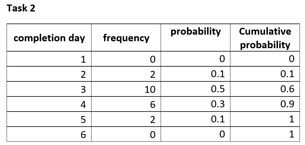
Assume the project has been carried a number of times in the past – say 20 times – and we have the data shown below for the two tasks. For each task, we have the frequency of completion by day. So, Task 1 was completed twice on day 3 , four times on day 4 and so on. Similarly, Task 2 was completed twice on the 2nd day after the task started and 10 times the 3rd day after the task started and so on.
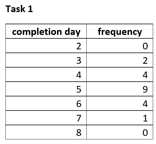

Consider Task 1. Since it was completed 2 times on day 3 and 4 times on day 4, it is reasonable to assume that it twice as likely that it will finish on day 4 than on day 3. In other words, the number of times a task is completed on a particular day is proportional to the probability of finishing on that day.
One can therefore approximate the probability of finishing on a particular day by dividing the number of completions on that day by the total number of times the task was performed. So, for example, the probability of finishing task 1 on day 3 is 2/20 or 0.1 and the probability of finishing it on day 4 is 0.2.
It is straightforward to calculate the probability for each of the completion days. The tables displayed below show the calculated probabilities. The tables also show the cumulative probability – this is sum of all probabilities of completion prior to (and including) current completion day. This gives the probability of finishing by the particular day – that is, on that day or any day before it. This, rather than the probability, is typically what you want to know.

The cumulative probability has two useful properties
- It is an increasing function (that is, it increases as the completion day increases)
- It lies between 0 and 1
What this means is that if we pick any number between 0 and 1, we will be able to find the “completion day” corresponding to that number. Let’s try this for task one:
Say we pick 0.35. Since 0.35 lies between 0.3 and 0.75, it corresponds to a completion between day 4 and day 5. That is, the task will be completed by day 5. Indeed, any number picked between 0.3 and 0.75 will correspond to a completion by day 5.
Say we pick 0.79. Since 0.79 lies between 0.75 and 0.95, it corresponds to a completion between day 5 and day 6. That is, the task will be completed by day 6.
….and so on. It is easy to see that any random number between 0 and 1 corresponds to a specific completion day depending on which cumulative probability interval it lies in.
Let’s pick a thousand random numbers between 0 and 1 and find the corresponding completion days for each. It should be clear from what I have said so far that these correspond to 1000 simulations of task 1, consistent with the historical data that we have on the task.
We will do the simulations in Excel. You may want to download the workbook that accompanies this post and follow along.
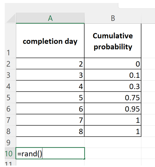
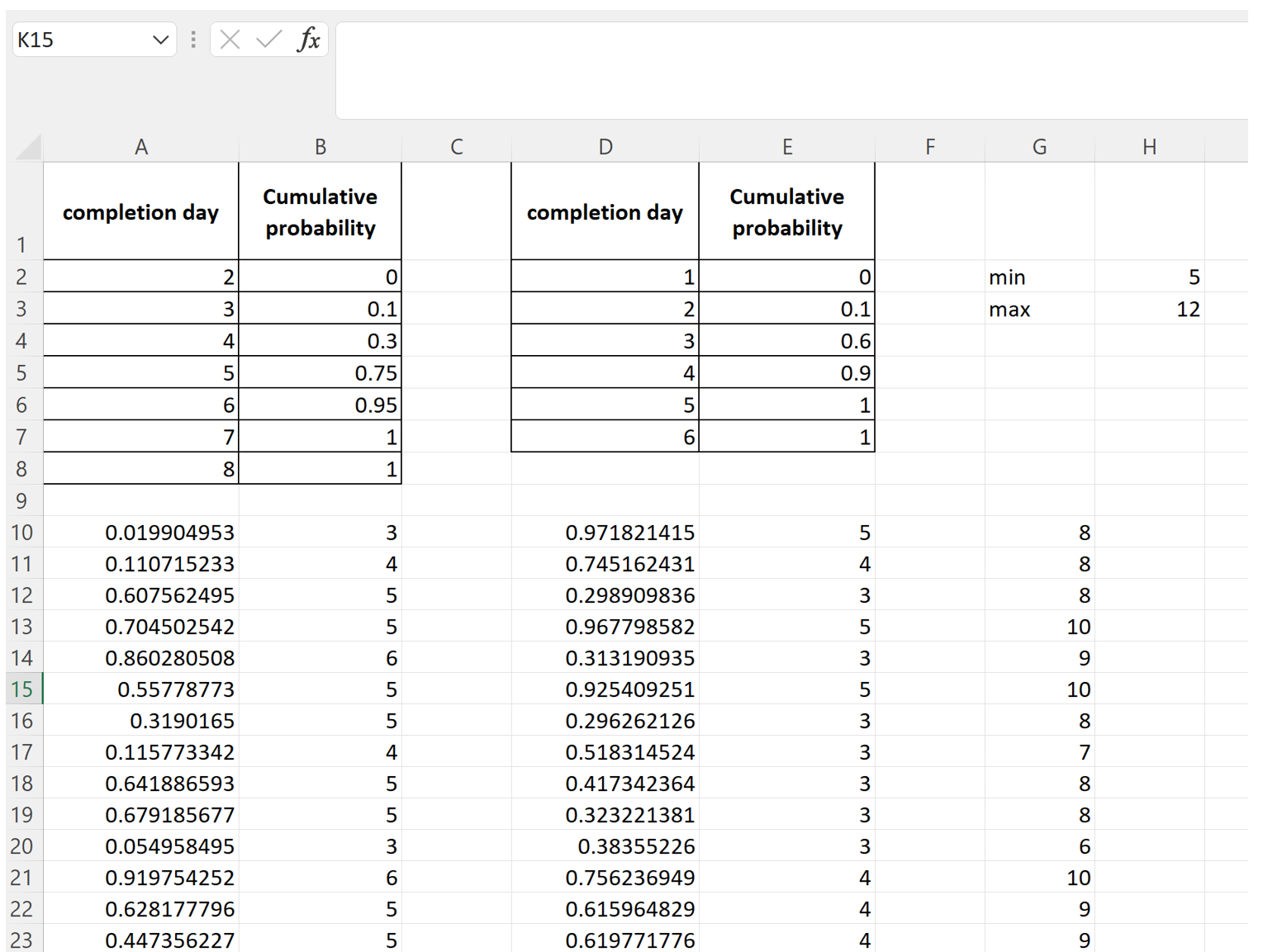
Enter the completion days and the cumulative probabilities corresponding to them in rows 1 through 8 of columns A and B as shown below.

Then enter the Excel RAND() function in cell A10 as shown in the figure below. This generates a random number between 0 and 1 (note that the random number you generate will be different from mine).
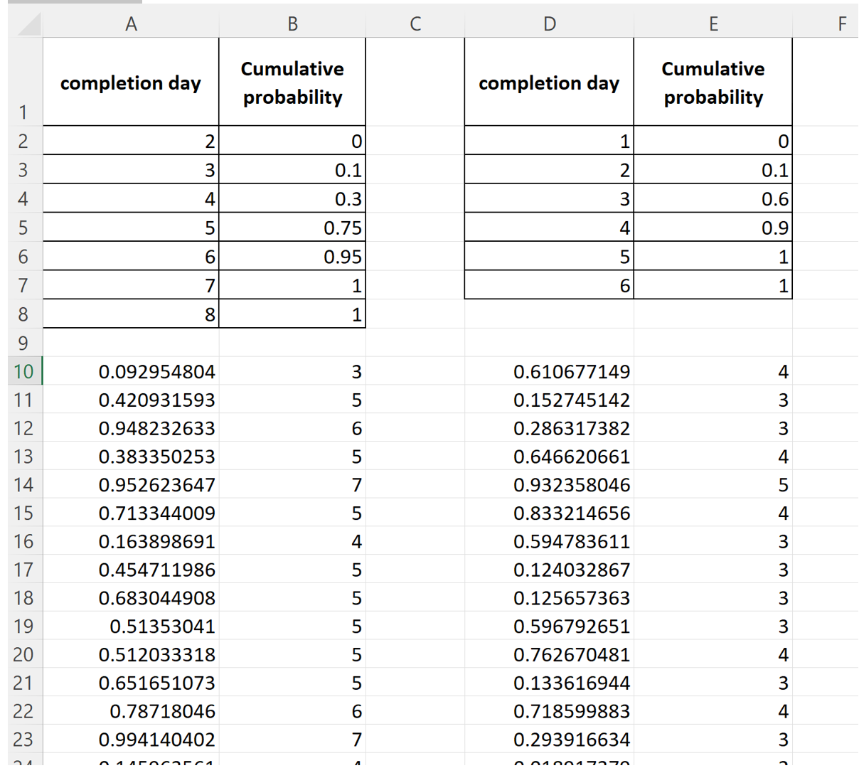
Next, fill down to cell A1009 to generate 1000 random numbers between 0 and 1 – see figure below ( again your random numbers will be different from mine)

Now in cell B10, input the formula shown below:

This nested IF() function checks which cumulative probability interval the random number lies in and returns the corresponding completion day. This is the completed by day corresponding to the inputted probability.
Fill this down to cell B1009. Your first few rows will look something like shown in the figure below:

You have now simulated Task 1 thousand times.
Next, enter the data for task 2 in columns D and E (from rows 1 through 7) and follow a similar procedure to simulate Task 2 thousand times. When you’re done, you will have something like what’s shown below (again, your random numbers and hence your completed by days will differ from mine):
Each line from row 10 to 1009 corresponds to a simulation of the project. So, this is equivalent to running the project 1000 times.
We can get completion times for each simulation by summing columns B and E, which will give us 1000 project completion times. Let’s do this in column G.
Using the MIN() and MAX() functions over the range G10:G1009, we see that the earliest and latest days for project completion are day 5 and day 12 respectively.
Using the simulation results, we can now get approximate cumulative probabilities for each of the possible completion days (i.e days 5 through 12).
Pause for a minute and have a think about how you would do this.
–x–
OK, so here’s how you would do it for day 5
Count the number of 5s in the range G10:G1009 using the COUNTIF() function. To estimate the probability of completion on day 5, divide this number by the total number of simulations.
To get the cumulative probability you would need to add in the probabilities for all prior completion days. However, since day 5 is the earliest possible completion day, there is no prior day.
Let’s do day 6
Count the number of 6s in the range G10:G1009 using the COUNTIF() function. To estimate the probability of completion on day 6, divide this number by the total number of simulations.
To get the cumulative probability you would need to add the estimated probability of completion for day 5 to the estimated probability of completion for day 6.
…and so on.
The resulting table, show below, is excerpted from columns J and K of the Excel workbook linked to above. Your numbers will differ (but hopefully by not too much) from the ones shown in the table.

Now that we have done all this work, we can make statements like:
- It is highly unlikely that we will finish before day 7.
- There’s an 80% chance that we will finish by day 9.
- There’s a 95% chance we’ll finish by day 10.
…and so on.
And that’s how Monte Carlo simulations work in the context of project estimation
Before we close, a word or two about data. The method we have used here assumes that you have detailed historical completion data for the tasks. However, you probably know from experience that it is rarely the case that you have this.
What do you do then?
Well, one can develop probability distributions based on subjective probabilities. Here’s how: ask the task performer for a best guess earliest, most likely and latest completion time. Based on these, one can construct triangular probability distributions that can be used in simulations. It would take me far too long to explain the procedure here so I’ll point you to an article instead.
And that’s it for this explainer. I hope it has given you a sense for how Monte Carlo simulations work.


