Probability | Eight to Late

Archive for the ‘Probability’ Category

The effect of task duration correlations on project schedules – a study using Monte Carlo simulation

Introduction

Some time ago, I wrote a couple of posts on Monte Carlo simulation of project tasks: the the first post presented a fairly detailed introduction to the technique and the second illustrated its use via three simple examples. The examples in the latter demonstrated the effect of various dependencies on overall completion times. The dependencies discussed were: two tasks in series (finish-to-start dependency), two tasks in series with a time delay (finish-to-start dependency with a lag) and two tasks in parallel (start-to-start dependency). All of these are dependencies in timing: i.e. they dictate when a successor task can start in relation to its predecessor. However, there are several practical situations in which task durations are correlated – that is, the duration of one task depends on the duration of another. As an example, a project manager working for an enterprise software company might notice that the longer it takes to elicit requirements the longer it takes to customise the software. When tasks are correlated thus, it is of interest to find out the effect of the correlation on the overall (project) completion time. In this post I explore the effect of correlations on project schedules via Monte Carlo simulation of a simple “project” consisting of two tasks in series.

A bit about what’s coming before we dive into it. I begin with a brief discusssion on how correlations are quantified. I then describe the simulation procedure, following which I present results for the example mentioned earlier, with and without correlations. I then present a detailed comparison of the results for the uncorrelated and correlated cases. It turns out that correlations increase uncertainty. This seemed counter-intuitive to me at first, but the simulations helped me see why it is so.

Note that I’ve attempted to keep the discussion intuitive and (largely) non-mathematical by relying on graphs and tables rather than formulae. There are a few formulae but most of these can be skipped quite safely.

Correlated project tasks

Imagine that there are two project tasks, A and B, which need to be performed sequentially. To keep things simple, I’ll assume that the durations of A and B are described by a triangular distribution with minimum, most likely and maximum completion times of 2, 4 and 8 days respectively (see my introductory Monte Carlo article for a detailed discussion of this distribution – note that I used hours as the unit of time in that post). In the absence of any other information, it is reasonable to assume that the durations of A and B are independent or uncorrelated – i.e. the time it takes to complete task A does not have any effect on the duration of task B. This assumption can be tested if we have historical data. So let’s assume we have the following historical data gathered from 10 projects:

Duration A (days))	duration B (days)
2.5	3
3	3
7	7.5
6	4.5
5.5	3.5
4.5	4.5
5	5.5
4	4.5
6	5
3	3.5

Figure 1 shows a plot of the duration of A vs. the duration of B. The plot suggests that there is a relationship between the two tasks – the longer A takes, the chances are that B will take longer too.

Figure 1: Duration of A vs. Duration of B

In technical terms we would say that A and B are positively correlated (if one decreased as the other increased, the correlation would be negative).

There are several measures of correlation, the most common one being Pearson’s coefficient of correlation $r$ which is given by

$r= \frac{\sum (x_{i} - \bar x)(y_{i}-\bar y)}{\sqrt{\sum (x_{i}-\bar x)^2}\sqrt{\sum (y_{i}-\bar y^2)}}\ldots\ldots (1)$

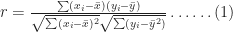
In this case $x_{i}$ and $y_{i}$ are the durations of the tasks A and B the $i$ th time the project was performed, $\bar x$ the average duration of A, $\bar y$ the average duration of B and $N$ the total number of data points (10 in this case). The capital sigma ( $\Sigma$ ) simply denotes a sum from 1 to N.

The Pearson coefficient, can vary between -1 and 1: the former being a perfect negative correlation and the latter a perfect positive one [Note: The Pearson coefficient is sometimes referred to as the product-moment correlation coefficient]. On calculating $r$ for the above data, using the CORREL function in Excel, I get a value of 0.787 (Note that one could just as well use the PEARSON function). This is a good indication that there is something going on here – the two tasks are likely not independent as originally assumed. Note that the correlation coefficient does not tell us anything about the form of the dependence between A and B; it only tells us that they are dependent and whether the dependence is positive or negative. It is also important to note that there is a difference between quantifying the correlation via the Pearson (or any other) coefficient and developing an understanding of why there is a correlation. The coefficient tells us nothing about the latter.

If A and B are correlated as discussed above, simulations which assume the tasks to be independent will not be correct. In the remainder of this article I’ll discuss how correlations affect overall task durations via a Monte Carlo simulation of the aforementioned example.

Simulating correlated project tasks

There are two considerations when simulating correlated tasks. The first is to characterize the correlation accurately. For the purposes of the present discussion I’ll assume that the correlation is described adequately by a single coefficient as discussed in the previous section. The second issue is to generate correlated completion times that satisfy the individual task duration distributions (Remember that the two tasks A and B have completion times that are described by a triangular distribution with minimum, maximum and most likely times of 2, 4 and 8 days). What we are asking for, in effect, is a way to generate a series of two correlated random numbers, each of which satisfy the triangular distribution.

The best known algorithm to generate correlated sets of random numbers in a way that preserves the individual (input) distributions is due to Iman and Conover. The beauty of the Iman-Conover algorithm is that it takes the uncorrelated data for tasks A and B (simulated separately) as input and induces the desired correlation by simply re-ordering the uncorrelated data. Since the original data is not changed, the distributions for A and B are preserved. Although the idea behind the method is simple, it is technically quite complex. The details of the technique aren’t important – but I offer a partial “hand-waving” explanation in the appendix at the end of this post. Fortunately I didn’t have to implement the Iman-Conover algorithm because someone else has done the hard work: Steve Roxburgh has written a graphical tool to generate sets of correlated random variables using the technique (follow this link to download the software and this one to view a brief tutorial) . I used Roxburgh’s utility to generate sets of random variables for my simulations.

I looked at two cases: the first with no correlation between A and B and the second with a correlation of 0.79 between A and B. Each simulation consisted of 10,000 trials – basically I generated two sets of 10,000 triangularly-distributed random numbers, the first with a correlation coefficient close to zero and the second with a correlation coefficient of 0.79. Figures 2 and 3 depict scatter plots of the durations of A vs. the durations of B (for the same trial) for the uncorrelated and correlated cases. The correlation is pretty clear to see in Figure 3.

Figure 2: Scatter plot of duration of A vs. duration of B (uncorrelated)

Figure 3: Scatter plot of duration of A vs. duration of B (correlated)

To check that the generated trials for A and B do indeed satisfy the triangular distribution, I divided the difference between the minimum and maximum times (for the individual tasks) into 0.5 day intervals and plotted the number of trials that fall into each interval. The resulting histograms are shown in Figure 4. Note that the blue and red bars are frequency plots for the case where A and B are uncorrelated and the green and pink (purple?) bars are for the case where they are correlated.

Figure 4: Frequency histograms for A and B (correlated and uncorrelated)

The histograms for all four cases are very similar, demonstrating that they all follow the specified triangular distribution. Figures 2 through 4 give confidence (but do not prove!) that Roxburgh’s utility works as advertised: i.e. that it generates sets of correlated random numbers in a way that preserves the desired distribution.

Now, to simulate A and B in sequence I simply added the durations of the individual tasks for each trial. I did this twice – once each for the correlated and uncorrelated data sets – which yielded two sets of completion times, varying between 4 days (the theoretical minimum) and 16 days (the theoretical maximum). As before, I plotted a frequency histogram for the uncorrelated and correlated case (see Figure 5). Note that the difference in the heights of the bars has no significance – it is an artefact of having the same number of trials (10,000) in both cases. What is significant is the difference in the spread of the two plots – the correlated case has a greater spread signifying an increased probability of very low and very high completion times compared to the uncorrelated case.

Figure 5: Frequency histograms for overall duration (blue=uncorrelated, red=correlated)

Note that the uncorrelated case resembles a Normal distribution – it is more symmetric than the original triangular distribution. This is a consequence of the Central Limit Theorem which states that the sum of identically distributed, independent (i.e. uncorrelated) random numbers is Normally distributed, regardless of the form of original distribution. The correlated distribution, on the other hand, has retained the shape of the original triangular distribution. This is no surprise: the relatively high correlation coefficient ensures that A and B will behave in a similar fashion and, hence, so will their sum.

Figure 6 is a plot of the cumulative distribution function (CDF) for the uncorrelated and correlated cases. The value of the CDFat any time $t$ gives the probability that the overall task will finish within time $t$ .

Figure 6: Cumulative probability distribution for uncorrelated (blue) and correlated (red) cases

The cumulative distribution clearly shows the greater spread in the correlated case: for small values of $t$ , the correlated distribution is significantly greater than the uncorrelated one; whereas for high values of $t$ , the correlated distribution approaches the limiting value of 1 more slowly than the uncorrelated distribution. Both these factors point to a greater spread in the correlated case. The spread can be quantified by looking at the standard deviation of the two distributions. The standard deviation, often denoted by the small greek letter sigma ( $\sigma$ ), is given by:

$\sigma =\sqrt{\frac{\sum (t_{i}-\bar t)^2}{N}} \ldots\ldots (2)$

wher $N$ is the total number of trials (10000), $t_{i}$ is the completion time for the $i$ th trial and $\bar t$ is the average completion time which is given by,

$\bar t= \frac{\sum t_{i}}{N} \ldots\ldots (3)$

In both (2) and (3) $\sum$ denotes a sum over all trials.

The averages, $\bar t$ , for the uncorrelated and correlated cases are virtually identical: 9.32 days and 9.34 days respectively. On the other hand, the standard deviations for the two cases are 1.77 and 2.34 respectively –demonstrating the wider spread in possible completion times for the correlated case. And, of course, a wider spread means greater uncertainty.

So, the simulations tell us that correlations increase uncertainty. Let’s try to understand why this happens. Basically, if tasks are correlated positively, they “track” each other: that is, if one takes a long time so will the other (with the same holding for short durations). The upshot of this is that the overall completion time tends to get “stretched” if the first task takes longer than average whereas it gets “compressed” if the first task finishes earlier than average. Since the net effect of stretching and compressing would balance out, we would expect the mean completion time (or any other measure of central tendency – such as the mode or median) to be relatively unaffected. However, because extremes are amplified, we would expect the spread of the distribution to increase.

Wrap-up

In this post I have highlighted the effect of task correlations on project schedules by comparing the results of simulations for two sequential tasks with and without correlations. The example shows that correlations can increase uncertainty. The mechanism is easy to understand: correlations tend to amplify extreme outcomes, thus increasing the spread in the resulting distribution. The effect of the correlation (compared to the uncorrelated case) can be quantified by comparing the standard deviations of the two cases.

Of course, quantifying correlations using a single number is simplistic – real life correlations have all kinds of complex dependencies. Nevertheless, it is a useful first step because it helps one develop an intuition for what might happen in more complicated cases: in hindsight it is easy to see that (positive) correlations will amplify extremes, but the simple model helped me really see it.

— —

Appendix – more on the Iman-Conover algorithm

Below I offer a hand-waving, half- explanation of how the technique works; those interested in a proper, technical explanation should see this paper by Simon Midenhall.

Before I launch off into my explanation, I’ll need to take a bit of a detour on coefficients of correlation. The title of Iman and Conover’s paper talks about rank correlation which is different from product-moment (or Pearson) correlation discussed in this post. A popular measure of rank correlation is the Spearman coefficient, $r_{s}$ , which is given by:

$r_{s} = 1-\frac{6\Sigma d_{i}^2}{N(N^2-1)}$

where $d_{i}$ is the rank difference between the duration of A and B on the $i$ th instance of the project. Note that rank is calculated relative to all the other instances of a particular task (A or B). This is best explained through the table below, which shows the ranks for all instances of task A and B from my earlier example (columns 3 and 4).

duration A (days)	duration B (days)	rank A	rank B	rank difference squared
2.5	3	1	1	0
3	3	2	1	1
7	7.5	10	10	0
6	4.5	8	5	9
5.5	3.5	7	3	16
4.5	4.5	5	5	0
5	5.5	6	9	9
4	4.5	4	5	1
6	5	8	8	0
3	3.5	2	3	1

Note that ties cause the subsequent number to be skipped.

The last column lists the rank differences, $d_{i}^2$ . The above can be used to calculate $r_{s}$ , which works out to 0.776 – which is quite close to the Pearson coefficient calculated earlier (0.787). In practical terms, the Spearman coefficient is often considered to be an approximation to the Pearson coefficient.

With that background about the rank correlation, we can now move on to a brief discussion of the Iman-Conover algorithm.

In essence, the Iman-Conover method relies on reordering the set of to-be-correlated variables to have the same rank order as a reference distribution which has the desired correlation. To paraphrase from Midenhall’s paper (my two cents in italics):

Given two samples of n values from known distributions X and Y (the triangular distributions for A and B in this case) and a desired correlation between them (of 0.78), first determine a sample from a reference distribution that has exactly the desired linear correlation (of 0.78). Then re-order the samples from X and Y to have the same rank order as the reference distribution. The output will be a sample with the correct (individual, triangular) distributions and with rank correlation coefficient equal to that of the reference distribution…. Since linear (Pearson) correlation and rank correlation are typically close, the output has approximately the desired correlation structure…

The idea is beautifully simple, but a problem remains. How does one calculate the required reference distribution? Unfortunately, this is a fairly technical affair for which I could not find a simple explanation – those interested in a proper, technical discussion of the technique should see Chapter 4 of Midenhall’s paper or the original paper by Iman and Conover.

For completeness I should note that some folks have criticised the use of the Iman-Conover algorithm on the grounds that it generates rank correlated random variables instead of Pearson correlated ones. This is a minor technicality which does not impact the main conclusion of this post: i.e. that correlations increase uncertainty.

Written by K

December 10, 2009 at 10:13 pm

Posted in Estimation, Monte Carlo Simulation, Probability, Project Management, Risk analysis, Statistics

Monte Carlo simulation of multiple project tasks – three examples and some general comments

with 23 comments

Introduction

In my previous post I demonstrated the use of a Monte Carlo technique in simulating a single project task with completion times described by a triangular distribution. My aim in that article was to: a) describe a Monte Carlo simulation procedure in enough detail for someone interested to be able to reproduce the calculations and b) show that it gives sensible results in a situation where the answer is known. Now it’s time to take things further. In this post, I present simulations for two tasks chained together in various ways. We shall see that, even with this small increase in complexity (from one task to two), the results obtained can be surprising. Specifically, small changes in inter-task dependencies can have a huge effect on the overall (two-task) completion time distribution. Although, this is something that that most project managers have experienced in real life, it is rarely taken in to account by traditional scheduling techniques. As we shall see, Monte Carlo techniques predict such effects as a matter of course.

Background

The three simulations discussed here are built on the example that I used in my previous article, so it’s worth spending a few lines for a brief recap of that example. The task simulated in the example was assumed to be described by a triangular distribution with minimum completion time ( $t_{min}$ ) of 2 hours, most likely completion time ( $t_{ml}$ ) of 4 hours and a maximum completion time ( $t_{max}$ ) of 8 hours. The resulting triangular probability distribution function (PDF), $p(t)$ – which gives the probability of completing the task at time t – is shown in Figure 1.

Figure 1 - PDF for triangular distribution (tmin=2, tml=4, tmax=8)

Figure 2 depicts the associated cumulative distribution function (CDF), $P(t)$ which gives the probability that a task will be completed by time t (as opposed to the PDF which specifies the probability of completion at time t). The value of the CDF at t=8 is 1 because the task must finish within 8 hrs.

Figure 2 - PDF for triangular distribution (tmin=2, tml=4, tmax=6)

The equations describing the PDF and CDF are listed in equations 4-7 of my previous article. I won’t rehash them here as they don’t add anything new to the discussion – please see the article for all the gory algebraic details and formulas. Now, with that background, we’re ready to move on to the examples.

Two tasks in series with no inter-task delay

As a first example, let’s look at two tasks that have to be performed sequentially – i.e. the second task starts as soon as the first one is completed. To simplify things, we’ll also assume that they have identical (triangular) distributions as described earlier and shown in Figure 1 (excepting , of course, that the distribution is shifted to the right for the second task – since it starts after the first one finishes). We’ll also assume that the second task begins right after the first one is completed (no inter-task delay) – yes, this is unrealistic, but bear with me. The simulation algorithm for the combined tasks is very similar to the one for a single task (described in detail in my previous post). Here’s the procedure:

For each of the two tasks, generate a set of N random numbers. Each random number generated corresponds to the cumulative probability of completion for a single task on that particular run.
For each random number generated, find the time corresponding to the cumulative probability by solving equation 6 or 7 in my previous post.
Step 2 gives N sets of completion times. Each set has two completion times – one for each tasks.
Add up the two numbers in each set to yield the comple. The resulting set corresponds to N simulation runs for the combined task.

I then divided the time interval from t=4 hours (min possible completion time for both tasks) to t=16 hours (max possible completion time for both tasks) into bins of 0.25 hrs each, and then assigned each combined completion time to the appropriate bin. For example, if the predicted completion time for a particular run was 9.806532 hrs, it was assigned to the bin corresponding to 0.975 hrs. The resulting histogram is shown in Figure 3 below (click on image to view the full-size graphic).

Figure 3 - Frequency histogram for tasks in series with no delay

Figure 3 - Frequency histogram for tasks in series with no inter-task delay

[An aside: compare the histogram in Figure 3 to the one for a single task (Figure 1): the distribution for the single task is distinctly asymmetric (the peak is not at the centre of the distribution) whereas the two task histogram is nearly symmetric. This surprising result is a consequence of the Central Limit Theorem (CLT) – which states that the sum of many identical distributions tends to resemble the Normal (Bell-shaped) distribution, regardless of the shape of the individual distributions. Note that the CLT holds even though the two task distributions are shifted relative to each other – i.e. the second task begins after the first one is completed.]

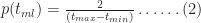
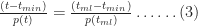
The simulation also enables us to compute the cumulative probability of completion for the combined tasks (the CDF). This value of the cumulative probability at a particular bin equals the sum of the number of simulations runs in every bin up to (and including) the bin in question, divided by the total number of simulation runs. In mathematical terms this is:

$P(t_{i})=(n_{1}+n_{2}+...+n_{i})/ N \ldots \ldots (1)$

where $P(t_{i})$ is the cumulative probability at the time corresponding to the $i$ th bin, $n_{i}$ , the number of simulation runs in the $i$ th bin and $N$ the total number of simulation runs. Note that this formula is an approximate one because time is treated as a constant within each bin. The approximation can be improved by making the bins smaller (and hence increasing the number of bins).

The resulting cumulative probability function is shown in Figure 4. This allows us to answer questions such as: “What is the probability that the tasks will be completed within 10 days?”. Answer: .698, or approximately 70%. (Note: I obtained this number by interpolating between values obtained from equation (1), but this level of precision is uncalled for, particularly because the formula is an approximate one)

Figure 4 - CDF for tasks in series with no inter-task delay

Many project scheduling techniques compute average completion times for component tasks and then add them up to get the expected completion time for the combined task. In the present case the average works out to 9.33 hrs (twice the average for a single task). However, we see from the CDF that there is a significant probability (.43) that we will not finish by this time – and this in a “best-case ” situation where the second task starts immediately after the first one finishes!

[An aside: If one applies the well-known PERT formula $(t_{min}+4t_{ml}+t_{max})/ 6$ to each of the tasks, one gets an expected completion time of 8.66 hrs for the combined task. From the CDF one can show that there is a probability of non-completion of 57% by t=8.66 hours (see Figure 4) – i.e. there’s a greater than even chance of not finishing by this time!]

As interesting as this case is, it is somewhat unrealistic because successor tasks seldom start the instant the predecessor is completed. More often than not, there is a cut-off time before which the successor cannot start – even if there are no explicit dependencies between the two tasks. This observation is a perfect segue into my next example, which is…

Two tasks in series with a fixed earliest start for the successor

Now we’ll introduce a slight complication: let’s assume, as before, that the two tasks are done one after the other but that the earliest the second task can start is at $t= 6$ hours (as measured from the start of the first task). So, if the first task finishes within 6 hours, there will be a delay between its completion and the start of the second task. However, if the first task takes longer than 6 hours to finish, the second task will start soon after the first one finishes. The simulation procedure is the same as described in the previous section excepting for the last step – the completion time for the combined task is given by:

$t=t_{1}+t_{2}$ , for t $\geq$ 6 hrs and $t=6+t_{2}$ , for t < 6 hrs

I divided the time interval from t=4hrs to t=20 hrs into bins of 0.25 hr duration (much as I did before) and then assigned each combined completion time to the appropriate bin. The resulting histogram is shown in Figure 5.

Figure 5 - Frequency histogram for tasks in series with inter-task delay

Comparing Figure 5 to Figure 3, we see that the earliest possible finish time now increases from 4 hrs to 8 hrs. This is no surprise, as we built this in to our assumption. Further, as one might expect, the distribution is distinctly asymmetric – with a minimum completion time of 8 hrs, a most likely time between 10 and 11 hrs and a maximum completion time of about 15 hrs.

Figure 6 shows the cumulative probability of completion for this case.

Figure 6 - CDF for tasks in series with inter-task delay

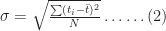
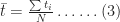
Because of the delay condition, it is impossible to calculate the average completion from the formulas for the triangular distribution – we have to obtain it from the simulation. The average can be calculated from the simulation adding up all completion times and dividing by the total number of simulations, $N$ . In mathematical terms this is:

$t_{av} = (t_{1} + t_{2} + ...+ t_{i} + ... + t_{N})/ N \ldots \ldots (2)$

where $t_{av}$ is the average time, $t_{i}$ the completion time for the $i$ th simulation run and $N$ the total number of simulation runs.

This procedure gave me a value of about 10.8 hrs for the average. From the CDF in Figure 6 one sees that the probability that the combined task will finish by this time is only 0.60 – i.e. there’s only a 60% chance that the task will finish by this time. Any naïve estimation of time would do just as badly unless, of course, one is overly pessimistic and assumes a completion time of 15 – 16 hrs.

From the above it should be evident that the simulation allows one to associate an uncertainty (or probability) with every estimate. If management imposes a time limit of 10 hours, the project manager can refer to the CDF in Figure 6 and figure out the probability of completing the task by that time (there’s a 40 % chance of completion by 10 hrs). Of course, the reliability of the numbers depend on how good the distribution is. But the assumptions that have gone into the model are known – the optimistic, most likely and pessimistic times and the form of the distribution – and these can be refined as one gains experience.

Two tasks in parallel

My final example is the case of two identical tasks performed in parallel. As above, I’ll assume the uncertainty in each task is characterized by a triangular distribution with $t_{min}$ , $t_{ml}$ and $t_{max}$ of 2, 4 and 8 hours respectively. The simulation procedure for this case is the same as in the first example, excepting the last step. Assuming the simulated completion times for the individual tasks are $t_{1}$ and $t_{2}$ , the completion time for the combined tasks is given by the greater of the two – i.e. the combined completion time $t$ is given by $t =max(t_{1},t_{2})$ .

To plot the histogram shown in Figure 7 , I divided the interval from t=2 hrs to t=8 hrs into bins of 0.25 hr duration each (Warning: Note the difference in the time axis scale from Figures 3 and 5!).

Figure 7 - Frequency histogram for tasks in parallel

It is interesting to compare the above histogram with that for an individual task with the same parameters (i.e. the example that was used in my previous post). Figure 8 shows the histograms for the two examples on the same plot (the combined task in red and the single task in blue). As one might expect, the histogram for the combined task is shifted to the right, a consequence of the nonlinear condition on the completion time.

Figure 8 - Histograms for tasks in parallel (red) and single task (blue)

What about the average? I calculated the average as before, by using equation (2) from the previous section. This gives an average of 5.38 hrs (compared to 4.67 hrs for either task, taken individually). Note that the method to calculate the average is the same regardless of the form of the distribution. On the other hand, computing the average from the equations would be a complicated affair, involving a stiff dose of algebra with an optional sprinkling of calculus. Even worse – the calculations would vary from distribution to distribution. There’s no question that simulations are much easier.

The CDF for the overall completion time is also computed easily using equation (1). The resulting plot is shown in Figure 9 (Note the difference in the time axis scale from Figures 4 and 6!). There are no surprises here – excepting how easy it is to calculate once the simulation is done.

Figure 9 - CDF for tasks in parallel

Let’s see what time corresponds to a 90% certainty of completion. A rough estimate for this number can be obtained from Figure 9 – just find the value of t (on the x axis) corresponding to a cumulative probability of 0.9 (on the y axis). This is the graphical equivalent of solving the CDF for time, given the cumulative probability is 0.9. From Figure 9, we get a time of approximately 6.7 hrs. [Note: we could get a more accurate number by fitting the points obtained from equation (1) to a curve and then calculating the time corresponding to $P=0.9$ ]. The interesting thing is that the 90% certain completion time is not too different from that of a single task (as calculated from equation 7 of my previous post) – which works out to 6.45 hrs.

Comparing the two histograms in Figure 8, we expect the biggest differences in cumulative probability to occur at about the t=4 hour mark, because by that time the probability for the individual task has peaked whereas that for the combined task is yet to peak. Let’s see if this is so: from Figure 8, the cumulative probability for t=4 hrs is about .15 and from the CDF for the triangular distribution (equation 6 from my previous post), the cumulative probability at t=4 hours (which is the most likely time) is .333 – double that of the combined task. This, again, isn’t too surprising (once one has Figure 8 on hand). The really nice thing is that we are able to attach uncertainties to all our estimates.

Conclusion

Although the examples discussed above are simple – two identical tasks with uncertainties described by a triangular distribution – they serve to illustrate some of the non-intuitive outcomes when tasks have dependencies. It is also worth noting that although the distribution for the individual tasks is known, the only straightforward way to obtain the distributions for the combined tasks (figures 3, 5 and 7) is through simulations. So, even these simple examples are a good demonstration of the utility of Monte Carlo techniques. Of course, real projects are way more complicated, with diverse tasks distributed in many different ways. To simplify simulations in such cases, one could perform coarse-grained simulations on a small number of high-level tasks, each consisting of a number of low-level, atomic tasks. The high-level tasks could be constructed in such a way as to focus attention on areas of greatest complexity, and hence greatest uncertainty.

As I have mentioned several times in this article and the previous one: simulation results are only as good as the distributions on which they are based. This begs the question: how do we know what’s an appropriate distribution for a given situation? There’s no one-size-fits-all answer to this question. However, for project tasks there are some general considerations that apply. These are:

There is a minimum time ( $t_{min}$ ) before which a task cannot cannot be completed.
The probability will increase from 0 at $t_{min}$ to a maximum at a “most likely” completion time, $t_{ml}$ . This holds true for most atomic tasks – but may be not for composite tasks which consist of many smaller tasks.
The probability decreases as time increases beyond $t_{ml}$ , falling to 0 at a time much larger than $t_{ml}$ . This is simply another way of saying that the distribution has a long (but not necessarily infinite!) tail.

Asymmetric triangular distributions (such as the one used in my examples) are the simplest distributions that satisfy these conditions. Furthermore, a three point estimate is enought to specify a triangular distribution completely – i.e. given a three point estimate there is only one triangular distribution that can be fitted to it. That said, there are several other distributions that can be used; of particular relevance are certain long-tailed distributions.

Finally, I should mention that I make no claims about the efficiency or accuracy of the method presented here: it should be seen as a demonstration rather than a definitive technique. The many commercial Monte Carlo tools available in the market probably offer far more comprehensive, sophisticated and reliable algorithms (Note: I ‘ve never used any of them, so I can’t make any recommendations!). That said, it is always helpful to know the principles behind such tools, if for no other reason than to understand how they work and, more important, how to use them correctly. The material discussed in this and the previous article came out of my efforts to develop an understanding Monte Carlo techniques and how they can be applied to various aspects of project management (they can also be applied to cost estimation, for example). Over the last few weeks I’ve spent many enjoyable evenings developing and running these simulations, and learning from them. I’ll leave it here with the hope that you find my articles helpful in your own explorations of the wonderful world of Monte Carlo simulations.

Written by K

September 20, 2009 at 9:34 pm

Posted in Estimation, Monte Carlo Simulation, portfolio management, Probability, Project Management, Statistics

An introduction to Monte Carlo simulation of project tasks

with 15 comments

Introduction

In an essay on the uncertainty of project task estimates, I described how a task estimate corresponds to a probability distribution. Put simply, a task estimate is actually a range of possible completion times, each with a probability of occurrence specified by a distribution. If one knows the distribution, it is possible to answer questions such as: “What is the probability that the task will be completed within x days?”

The reliability of such predictions depends on how faithfully the distribution captures the actual spread of task durations – and therein lie at least a couple of problems. First, the probability distributions for task durations are generally hard to characterise because of the lack of reliable data (estimators are not very good at estimating, and historical data is usually not available). Second, many realistic distributions have complicated mathematical forms which can be hard to characterise and manipulate.

These problems are compounded by the fact that projects consist of several tasks, each one with its own duration estimate and (possibly complicated) distribution. The first issue is usually addressed by fitting distributions to point estimates (such as optimistic, pessimistic and most likely times as in PERT) and then refining these estimates and distributions as one gains experience. The second issue can be tackled by Monte Carlo techniques, which involve simulating the task a number of times (using an appropriate distribution) and then calculating expected completion times based on the results. My aim in this post is to present an example-based introduction to Monte Carlo simulation of project task durations.

Although my aim is to keep things reasonably simple (not too much beyond high-school maths and a basic understanding of probability), I’ll be covering a fair bit of ground. Given this, I’d best to start with a brief description of my approach so that my readers know what coming.

Monte Carlo simulation is an umbrella term that covers a range of approaches that use random sampling to simulate events that are described by known probability distributions. The first task then, is to specify the probability distribution. However, as mentioned earlier, this is generally unknown for task durations. For simplicity, I’ll assume that task duration uncertainty can be described accurately using a triangular probability distribution – a distribution that is particularly easy to handle from the mathematical point of view. The advantage of using the triangular distribution is that simulation results can be validated easily.

Using the triangular distribution isn’t a limitation because the method I describe can be applied to arbitrarily shaped distributions. More important, the technique can be used to simulate what happens when multiple tasks are strung together as in a project schedule (I’ll cover this in a future post). Finally, I’ll demonstrate a Monte Carlo simulation method as applied to a single task described by a triangular distribution. Although a simulation is overkill in this case (because questions regarding durations can be answered exactly without using a simulation), the example serves to illustrate the steps involved in simulating more complex cases – such as those comprising of more than one task and/or involving more complicated distributions.

So, without further ado, let me begin the journey by describing the triangular distribution.

The triangular distribution

Let’s assume that there’s a project task that needs doing, and the person who is going to do it reckons it will take between 2 and 8 hours to complete it, with a most likely completion time of 4 hours. How the estimator comes up with these numbers isn’t important at this stage – maybe there’s some guesswork, maybe some padding or maybe it is really based on experience (as it should be). What’s important is that we have three numbers corresponding to a minimum, most likely and maximum time. To keep the discussion general, we’ll call these $t_{min}$ , $t_{ml}$ and $t_{max}$ respectively, (we’ll get back to our estimator’s specific numbers later).

Now, what about the probabilities associated with each of these times?

Since $t_{min}$ and $t_{max}$ correspond to the minimum and maximum times, the probability associated with these is zero. Why? Because if it wasn’t zero, then there would be a non-zero probability of completion for a time less than $t_{min}$ or greater than $t_{max}$ – which isn’t possible [Note: this is a consequence of the assumption that the probability varies continuously – so if it takes on non-zero value, $p_{0}$ , at $t_{min}$ then it must take on a value slightly less than $p_{0}$ – but greater than 0 – at $t$ slightly smaller than $t_{min}$ ] . As far as the most likely time, $t_{ml}$ , is concerned: by definition, the probability attains its highest value at time $t_{ml}$ . So, assuming the probability can be described by a triangular function, the distribution must have the form shown in Figure 1 below.

Figure 1: Triangular Distribution

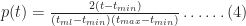
For the simulation, we need to know the equation describing the above distribution. Although Wikipedia will tell us the answer in a mouse-click, it is instructive to figure it out for ourselves. First, note that the area under the triangle must be equal to 1 because the task must finish at some time between $t_{min}$ and $t_{max}$ . As a consequence we have:

$\frac{1}{2}\times{base}\times{altitude}=\frac{1}{2}\times{(t_{max}-t_{min})}\times{p(t_{ml})}=1\ldots\ldots{(1)}$

where $p(t_{ml})$ is the probability corresponding to time $t_{ml}$ . With a bit of rearranging we get,

$p(t_{ml})=\frac{2}{(t_{max}-t_{min})}\ldots\ldots(2)$

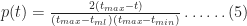
To derive the probability for any time $t$ lying between $t_{max}$ and $t_{ml}$ , we note that:

$\frac{(t-t_{min})}{p(t)}=\frac{(t_{ml}-t_{min})}{p(t_{ml})}\ldots\ldots(3)$

This is a consequence of the fact that the ratios on either side of equation (3) are equal to the slope of the line joining the points $(t_{min},0)$ and $(t_{ml}, p(t_{ml}))$ .

Figure 2

Substituting (2) in (3) and simplifying a bit, we obtain:

$p(t)=\frac{2(t-t_{min})}{(t_{ml}-t_{min})(t_{max}-t_{min})}\dots\ldots(4)$ for $t_{min}\leq t \leq t_{ml}$

In a similar fashion one can show that the probability for times lying between $t_{ml}$ and $t_{max}$ is given by:

$p(t)=\frac{2(t_{max}-t)}{(t_{max}-t_{ml})(t_{max}-t_{min})}\dots\ldots(5)$ for $t_{ml}\leq t \leq t_{max}$

Equations 4 and 5 together describe the probability distribution function (or PDF) for all times between $t_{min}$ and $t_{max}$ .

Another quantity of interest is the cumulative distribution function (or CDF) which is the probability, $P$ , that the task is completed by a time $t$ . To reiterate, the PDF, $p(t)$ , is the probability of the task finishing at time $t$ whereas the CDF, $P(t)$ , is the probability of the task completing by time $t$ . The CDF, $P(t)$ , is essentially a sum of all probabilities between $t_{min}$ and $t$ . For $t < t_{min}$ this is the area under the triangle with apexes at ( $t_{min}$ , 0), (t, 0) and (t, p(t)). Using the formula for the area of a triangle (1/2 base times height) and equation (4) we get:

$P(t)=\frac{(t-t_{min})^2}{(t_{ml}-t_{min})(t_{max}-t_{min})}\ldots\ldots(6)$ for $t_{min}\leq t \leq t_{ml}$

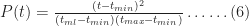
Noting that for $t \geq t_{ml}$ , the area under the curve equals the total area minus the area enclosed by the triangle with base between t and $t_{max}$ , we have:

$P(t)=1- \frac{(t_{max}-t)^2}{(t_{max}-t_{ml})(t_{max}-t_{min})}\ldots\ldots(7)$ for $t_{ml}\leq t \leq t_{max}$

As expected, $P(t)$ starts out with a value 0 at $t_{min}$ and then increases monotonically, attaining a value of 1 at $t_{max}$ .

To end this section let's plug in the numbers quoted by our estimator at the start of this section: $t_{min}=2$ , $t_{ml}=4$ and $t_{max}=8$ . The resulting PDF and CDF are shown in figures 3 and 4.

Figure 3 - Triangular PDF (tmin=2, tml=4, tmax=8)

Figure 4 – Triangular CDF (tmin=2, tml=4, tmax=8)

Monte Carlo Simulation of a Single Task

OK, so now we get to the business end of this essay – the simulation. I’ll first outline the simulation procedure and then discuss results for the case of the task described in the previous section (triangular distribution with $t_{min}=2$ , $t_{ml}=4$ and $t_{max}=8$ ). Note that I used TK Solver – a mathematical package created by Universal Technical Systems – to do the simulations. TK Solver has built-in backsolving capability which is extremely helpful for solving some of the equations that come up in the simulation calculations. One could use Excel too, but my spreadsheet skills are not up to it :-(.

So, here’s my simulation procedure:

Generate a random number between 0 and 1. Treat this number as the cumulative probability, $P(t)$ for the simulation run. [Technical Note: I used the random number generator that comes with the TK Solver package (the algorithm used by the generator is described here). Excel’s random number generator is even better.]
Find the time, $t$ , corresponding to $P(t)$ by solving equations (6) or (7) for $t$ . The resulting value of $t$ is the time taken to complete the task. [Technical Note: Solving equation (6) or (7) for $t$ isn’t straightforward because $t$ appears in several places in the equations. One has two options to solve for $t$ a) Use numerical techniques such as the bisection or Newton-Raphson method or b) use the backsolve (goal seek) functionality in Excel or other mathematical packages. I used the backsolving capability of TK Solver to obtain t for each random value of P generated. TK Solver backsolves equations automatically – no fiddling around with numerical methods – which makes it an attractive option for these kinds of calculations.]
Repeat steps (1) and (2) N times, where N is a “sufficiently large” number – say 10,000.

I did the calculations for $N=10000$ using the triangular distribution with parameters $t_{min}=2$ , $t_{ml}=4$ and $t_{max}=8$ . This gave me 10,000 values of $P(t)$ and $t$ .

As an example of a simulation run proceeds, here’s the data from my first simulation run: the random number generator returned 0.490474700804856 (call it 0.4905). This is the value of $P(t)$ . The time corresponding to this cumulative probability is obtained by solving equation (7) numerically for $t$ . This gave $t = 4.503057452476027$ (call it 4.503) as shown in Figure 5. This is the completion time for the first run.

Figure 5

After completing 10,000 simulation runs, I sorted these into bins corresponding to time intervals of .25 hrs, starting from $t$ =2hrs through to $t$ =8 hrs. The resulting histogram is shown in Figure 6. Each bar corresponds to the number of simulation runs that fall within that time interval.

Figure 6: Distribution of simulation runs

As one might expect, this looks like the triangular distribution shown in Figure 4. There is a difference though: Figure 4 plots probability as a continuous function of time whereas Figure 6 plots the number of simulation runs as a step function of time. To convince ourselves that the two are really the same, lets look at the cumulative probability at $t_{ml}$ – i.e the probability that the task will be completed within 4 hrs. From equation 6 we get $P(t_{ml})=0.3333$ . The corresponding number from the simulation is simply the number of simulation runs that had a completion time less than or equal to 4 hrs, divided by the total number of simulation runs. For my simulation this comes out to be 0.3383. The agreement’s not perfect, but is convincing enough. Just to be sure, I performed the simulation a number of times – generating several sets of random numbers – and took the average of the predicted $P(t_{ml})$ . The agreement between theory and simulation improved, as expected.

Wrap up

A limitation of the triangular distribution is that it imposes an upper cut-off at $t_{max}$ . Long-tailed distributions may therefore be more realistic. In the end, though, the form distribution is neither here nor there because the technique can be applied to any distribution. The real question is: how do we obtain reliable distributions for our estimates? There’s no easy answer to this one, but one can start with three point estimates (as in PERT) and then fit these to a triangular (or more complicated) distribution. Although it is best if one has historical data, in the absence this one can always start with reasonable guesses. The point is to refine these through experience.

Another point worth mentioning is that simulations can be done at a level higher than that of an indivdual task. In their brilliant book – Waltzing With Bears: Managing Risk on Software Projects – De Marco and Lister demonstrate the use of Monte Carlo methods to simulate various aspects of project – velocity, time, cost etc. – at the project level (as opposed to the task level). I believe it is better to perform simulations at the lowest possible level (although it is a lot more work) – the main reason being that it is easier, and less error-prone, to estimate individual tasks than entire projects. Nevertheless, high level simulations can be very useful if one has reliable data to base these on.

I would be remiss if I didn’t mention some of the various Monte Carlo packages available in the market. I’ve never used any of these, but by all accounts they’re pretty good: see this commercial package or this one, for example. Both products use random number generators and sampling techniques that are far more sophisticated than the simple ones I’ve used in my example.

Finally, I have to admit that the example described in this post is a very complicated way of demonstrating the obvious – I started out with the triangular distribution and then got back the triangular distribution via simulation. My point, however, was to illustrate the method and show that it yields expected results in a situation where the answer is known. In a future post I’ll apply the method to more complex situations- for example, multiple tasks in series and parallel, with some dependency rules thrown in for good measure. Although, I’ll use the triangular distribution for individual tasks, the results will be far from obvious: simulation methods really start to shine as complexity increases. But all that will have to wait for later. For now, I hope my example has helped illustrate how Monte Carlo methods can be used to simulate project tasks.

Note added on 21 Sept 2009:

Follow-up to this article published here.

Note added on 14 Dec 2009:

See this post for a Monte Carlo simulation of correlated project tasks.

Written by K

September 11, 2009 at 11:05 pm

Posted in Estimation, Monte Carlo Simulation, portfolio management, Probability, Project Management, Statistics

Eight to Late

Archive for the ‘Probability’ Category

The effect of task duration correlations on project schedules – a study using Monte Carlo simulation

Introduction

Correlated project tasks

Simulating correlated project tasks

Wrap-up

Appendix – more on the Iman-Conover algorithm

Monte Carlo simulation of multiple project tasks – three examples and some general comments

Introduction

Background

Two tasks in series with no inter-task delay

Two tasks in series with a fixed earliest start for the successor

Two tasks in parallel

Conclusion

An introduction to Monte Carlo simulation of project tasks

Introduction

The triangular distribution

Monte Carlo Simulation of a Single Task

Wrap up

Subscribe

Search

Author

Copyright

My book

Top Posts & Pages

Recent Posts

Categories

Archives

Blogroll

Other links

Eight to Late

Archive for the ‘Probability’ Category

The effect of task duration correlations on project schedules – a study using Monte Carlo simulation

Introduction

Correlated project tasks

Simulating correlated project tasks

Wrap-up

Appendix – more on the Iman-Conover algorithm

Rate this:

Share this:

Monte Carlo simulation of multiple project tasks – three examples and some general comments

Introduction

Background

Two tasks in series with no inter-task delay

Two tasks in series with a fixed earliest start for the successor

Two tasks in parallel

Conclusion

Rate this:

Share this:

An introduction to Monte Carlo simulation of project tasks

Introduction

The triangular distribution

Monte Carlo Simulation of a Single Task

Wrap up

Rate this:

Share this:

Subscribe

Search

Author

Copyright

My book

Top Posts & Pages

Recent Posts

Categories

Archives

Blogroll

Other links