The effect of task duration correlations on project schedules – a study using Monte Carlo simulation
Introduction
Some time ago, I wrote a couple of posts on Monte Carlo simulation of project tasks: the the first post presented a fairly detailed introduction to the technique and the second illustrated its use via three simple examples. The examples in the latter demonstrated the effect of various dependencies on overall completion times. The dependencies discussed were: two tasks in series (finish-to-start dependency), two tasks in series with a time delay (finish-to-start dependency with a lag) and two tasks in parallel (start-to-start dependency). All of these are dependencies in timing: i.e. they dictate when a successor task can start in relation to its predecessor. However, there are several practical situations in which task durations are correlated – that is, the duration of one task depends on the duration of another. As an example, a project manager working for an enterprise software company might notice that the longer it takes to elicit requirements the longer it takes to customise the software. When tasks are correlated thus, it is of interest to find out the effect of the correlation on the overall (project) completion time. In this post I explore the effect of correlations on project schedules via Monte Carlo simulation of a simple “project” consisting of two tasks in series.
A bit about what’s coming before we dive into it. I begin with a brief discusssion on how correlations are quantified. I then describe the simulation procedure, following which I present results for the example mentioned earlier, with and without correlations. I then present a detailed comparison of the results for the uncorrelated and correlated cases. It turns out that correlations increase uncertainty. This seemed counter-intuitive to me at first, but the simulations helped me see why it is so.
Note that I’ve attempted to keep the discussion intuitive and (largely) non-mathematical by relying on graphs and tables rather than formulae. There are a few formulae but most of these can be skipped quite safely.
Correlated project tasks
Imagine that there are two project tasks, A and B, which need to be performed sequentially. To keep things simple, I’ll assume that the durations of A and B are described by a triangular distribution with minimum, most likely and maximum completion times of 2, 4 and 8 days respectively (see my introductory Monte Carlo article for a detailed discussion of this distribution – note that I used hours as the unit of time in that post). In the absence of any other information, it is reasonable to assume that the durations of A and B are independent or uncorrelated – i.e. the time it takes to complete task A does not have any effect on the duration of task B. This assumption can be tested if we have historical data. So let’s assume we have the following historical data gathered from 10 projects:
| Duration A (days)) | duration B (days) |
| 2.5 | 3 |
| 3 | 3 |
| 7 | 7.5 |
| 6 | 4.5 |
| 5.5 | 3.5 |
| 4.5 | 4.5 |
| 5 | 5.5 |
| 4 | 4.5 |
| 6 | 5 |
| 3 | 3.5 |
Figure 1 shows a plot of the duration of A vs. the duration of B. The plot suggests that there is a relationship between the two tasks – the longer A takes, the chances are that B will take longer too.

Figure 1: Duration of A vs. Duration of B
In technical terms we would say that A and B are positively correlated (if one decreased as the other increased, the correlation would be negative).
There are several measures of correlation, the most common one being Pearson’s coefficient of correlation 
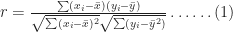
In this case 


The Pearson coefficient, can vary between -1 and 1: the former being a perfect negative correlation and the latter a perfect positive one [Note: The Pearson coefficient is sometimes referred to as the product-moment correlation coefficient]. On calculating
If A and B are correlated as discussed above, simulations which assume the tasks to be independent will not be correct. In the remainder of this article I’ll discuss how correlations affect overall task durations via a Monte Carlo simulation of the aforementioned example.
Simulating correlated project tasks
There are two considerations when simulating correlated tasks. The first is to characterize the correlation accurately. For the purposes of the present discussion I’ll assume that the correlation is described adequately by a single coefficient as discussed in the previous section. The second issue is to generate correlated completion times that satisfy the individual task duration distributions (Remember that the two tasks A and B have completion times that are described by a triangular distribution with minimum, maximum and most likely times of 2, 4 and 8 days). What we are asking for, in effect, is a way to generate a series of two correlated random numbers, each of which satisfy the triangular distribution.
The best known algorithm to generate correlated sets of random numbers in a way that preserves the individual (input) distributions is due to Iman and Conover. The beauty of the Iman-Conover algorithm is that it takes the uncorrelated data for tasks A and B (simulated separately) as input and induces the desired correlation by simply re-ordering the uncorrelated data. Since the original data is not changed, the distributions for A and B are preserved. Although the idea behind the method is simple, it is technically quite complex. The details of the technique aren’t important – but I offer a partial “hand-waving” explanation in the appendix at the end of this post. Fortunately I didn’t have to implement the Iman-Conover algorithm because someone else has done the hard work: Steve Roxburgh has written a graphical tool to generate sets of correlated random variables using the technique (follow this link to download the software and this one to view a brief tutorial) . I used Roxburgh’s utility to generate sets of random variables for my simulations.
I looked at two cases: the first with no correlation between A and B and the second with a correlation of 0.79 between A and B. Each simulation consisted of 10,000 trials – basically I generated two sets of 10,000 triangularly-distributed random numbers, the first with a correlation coefficient close to zero and the second with a correlation coefficient of 0.79. Figures 2 and 3 depict scatter plots of the durations of A vs. the durations of B (for the same trial) for the uncorrelated and correlated cases. The correlation is pretty clear to see in Figure 3.

Figure 2: Scatter plot of duration of A vs. duration of B (uncorrelated)

Figure 3: Scatter plot of duration of A vs. duration of B (correlated)
To check that the generated trials for A and B do indeed satisfy the triangular distribution, I divided the difference between the minimum and maximum times (for the individual tasks) into 0.5 day intervals and plotted the number of trials that fall into each interval. The resulting histograms are shown in Figure 4. Note that the blue and red bars are frequency plots for the case where A and B are uncorrelated and the green and pink (purple?) bars are for the case where they are correlated.

Figure 4: Frequency histograms for A and B (correlated and uncorrelated)
The histograms for all four cases are very similar, demonstrating that they all follow the specified triangular distribution. Figures 2 through 4 give confidence (but do not prove!) that Roxburgh’s utility works as advertised: i.e. that it generates sets of correlated random numbers in a way that preserves the desired distribution.
Now, to simulate A and B in sequence I simply added the durations of the individual tasks for each trial. I did this twice – once each for the correlated and uncorrelated data sets – which yielded two sets of completion times, varying between 4 days (the theoretical minimum) and 16 days (the theoretical maximum). As before, I plotted a frequency histogram for the uncorrelated and correlated case (see Figure 5). Note that the difference in the heights of the bars has no significance – it is an artefact of having the same number of trials (10,000) in both cases. What is significant is the difference in the spread of the two plots – the correlated case has a greater spread signifying an increased probability of very low and very high completion times compared to the uncorrelated case.

Figure 5: Frequency histograms for overall duration (blue=uncorrelated, red=correlated)
Note that the uncorrelated case resembles a Normal distribution – it is more symmetric than the original triangular distribution. This is a consequence of the Central Limit Theorem which states that the sum of identically distributed, independent (i.e. uncorrelated) random numbers is Normally distributed, regardless of the form of original distribution. The correlated distribution, on the other hand, has retained the shape of the original triangular distribution. This is no surprise: the relatively high correlation coefficient ensures that A and B will behave in a similar fashion and, hence, so will their sum.
Figure 6 is a plot of the cumulative distribution function (CDF) for the uncorrelated and correlated cases. The value of the CDFat any time 

Figure 6: Cumulative probability distribution for uncorrelated (blue) and correlated (red) cases
The cumulative distribution clearly shows the greater spread in the correlated case: for small values of 
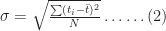
wher 

In both (2) and (3) 
The averages,
So, the simulations tell us that correlations increase uncertainty. Let’s try to understand why this happens. Basically, if tasks are correlated positively, they “track” each other: that is, if one takes a long time so will the other (with the same holding for short durations). The upshot of this is that the overall completion time tends to get “stretched” if the first task takes longer than average whereas it gets “compressed” if the first task finishes earlier than average. Since the net effect of stretching and compressing would balance out, we would expect the mean completion time (or any other measure of central tendency – such as the mode or median) to be relatively unaffected. However, because extremes are amplified, we would expect the spread of the distribution to increase.
Wrap-up
In this post I have highlighted the effect of task correlations on project schedules by comparing the results of simulations for two sequential tasks with and without correlations. The example shows that correlations can increase uncertainty. The mechanism is easy to understand: correlations tend to amplify extreme outcomes, thus increasing the spread in the resulting distribution. The effect of the correlation (compared to the uncorrelated case) can be quantified by comparing the standard deviations of the two cases.
Of course, quantifying correlations using a single number is simplistic – real life correlations have all kinds of complex dependencies. Nevertheless, it is a useful first step because it helps one develop an intuition for what might happen in more complicated cases: in hindsight it is easy to see that (positive) correlations will amplify extremes, but the simple model helped me really see it.
— —
Appendix – more on the Iman-Conover algorithm
Below I offer a hand-waving, half- explanation of how the technique works; those interested in a proper, technical explanation should see this paper by Simon Midenhall.
Before I launch off into my explanation, I’ll need to take a bit of a detour on coefficients of correlation. The title of Iman and Conover’s paper talks about rank correlation which is different from product-moment (or Pearson) correlation discussed in this post. A popular measure of rank correlation is the Spearman coefficient, 

where 
| duration A (days) | duration B (days) | rank A | rank B | rank difference squared |
| 2.5 | 3 | 1 | 1 | 0 |
| 3 | 3 | 2 | 1 | 1 |
| 7 | 7.5 | 10 | 10 | 0 |
| 6 | 4.5 | 8 | 5 | 9 |
| 5.5 | 3.5 | 7 | 3 | 16 |
| 4.5 | 4.5 | 5 | 5 | 0 |
| 5 | 5.5 | 6 | 9 | 9 |
| 4 | 4.5 | 4 | 5 | 1 |
| 6 | 5 | 8 | 8 | 0 |
| 3 | 3.5 | 2 | 3 | 1 |
Note that ties cause the subsequent number to be skipped.
The last column lists the rank differences, 
With that background about the rank correlation, we can now move on to a brief discussion of the Iman-Conover algorithm.
In essence, the Iman-Conover method relies on reordering the set of to-be-correlated variables to have the same rank order as a reference distribution which has the desired correlation. To paraphrase from Midenhall’s paper (my two cents in italics):
Given two samples of n values from known distributions X and Y (the triangular distributions for A and B in this case) and a desired correlation between them (of 0.78), first determine a sample from a reference distribution that has exactly the desired linear correlation (of 0.78). Then re-order the samples from X and Y to have the same rank order as the reference distribution. The output will be a sample with the correct (individual, triangular) distributions and with rank correlation coefficient equal to that of the reference distribution…. Since linear (Pearson) correlation and rank correlation are typically close, the output has approximately the desired correlation structure…
The idea is beautifully simple, but a problem remains. How does one calculate the required reference distribution? Unfortunately, this is a fairly technical affair for which I could not find a simple explanation – those interested in a proper, technical discussion of the technique should see Chapter 4 of Midenhall’s paper or the original paper by Iman and Conover.
For completeness I should note that some folks have criticised the use of the Iman-Conover algorithm on the grounds that it generates rank correlated random variables instead of Pearson correlated ones. This is a minor technicality which does not impact the main conclusion of this post: i.e. that correlations increase uncertainty.
Cooperation versus self-interest: the theory of collective action and its relevance to project management
Introduction
Conventional wisdom deems that any organizational activity involving several people has to be closely supervised to prevent it from dissolving into chaos and anarchy. The assumption underlying this view is that individuals involved in the activity will, if left unsupervised, make decisions based on self interest rather than the common good, and hence will invariably make the wrong decision as far as the collective enterprise is concerned. This assumption finds justification in rational choice theory, which predicts that individuals will act in ways that maximize their personal benefit without any regard to the common good. This view is exemplified in the so-called Tragedy of the Commons, where individuals who have access to a common resource over-exploit it in their pursuit of personal gain, and thus end up depleting the resource completely. Fortunately, this view is demonstrably incorrect: the work of Elinor Ostrom, one of the 2009 Nobel prize winners for Economics, shows that, given the right conditions, groups can work towards the common good even if it means forgoing personal gains. This post is a brief look into Ostrom’s work and the insights it offers into the theory and practice of project management.
Background: rationality, bounded rationality and theories of choice
Classical economics assumes that individuals’ actions are driven by rational self-interest – i.e. the well-known “what’s in it for me” factor (this is one of the assumptions of rational choice theory). So, in a situation where an individual has access to a resource that is also available to others, classical economics predicts that the individual will aim to maximize his or her benefit without any regard to the common good. Clearly, the group will achieve much better results as a whole if it were to exploit the resource in a cooperative way. There are several real-world examples where such cooperative behaviour has been successful in achieving outcomes for the common good (see this paper for some). However, according to classical economic theory, such cooperative behaviour is simply not possible.
So, what’s wrong with rational choice theory?
A couple of things, at least:
Firstly, implicit in rational choice theory is the assumption that individuals can figure out the best choice in any given situation. This is obviously incorrect. As Ostrom has stated in one of her papers:
Because individuals are boundedly rational, they do not calculate a complete set of strategies for every situation they face. Few situations in life generate information about all potential actions that one can take, all outcomes that can be obtained, and all strategies that others can take.
Instead, they use heuristics (experienced-based methods), norms (value-based techniques) and rules (mutually agreed regulations) to arrive at “good enough” decisions. Note that Ostrom makes a distinction between norms and rules, the former being implicit (unstated) rules, which are determined by the cultural attitudes and values)
Secondly, rational choice theory assumes that humans behave as self-centered, short-term maximisers. Such theories – which assume that humans act solely out of self interest – work in competitive situations (such as the stock-market) but do not work in situations in which collective action is called for.
Ostrom’s work essentially addresses the shortcomings of rational choice theory.
A behavioural approach
Ostrom’s work looks at how groups act collectively to solve social dilemmas such as the one implicit in the tragedy of the commons. To quote from this post by Umair Haque:
…Ostrom’s work is concerned, fundamentally, with challenging Garret Hardin’s famous, Tragedy of the Commons [Note: Hardin’s article can be accessed here], itself a living expression of neoclassical thinking. Ostrom suggests that far from a tragedy, the commons can be managed from the bottom-up for a shared prosperity — given the right institutions….
In a paper entitled, A Behavioral Approach to the Rational Choice Theory of Collective Action, published in 1998, Ostrom states that:
…much of our current public policy analysis is based on an assumption that rational individuals are helplessly trapped in social dilemmas from which they cannot extract themselves without inducement or sanctions applied from the outside. Many policies based on this assumption have been subject to major failure and have exacerbated the very problems they were in-tended to ameliorate. Policies based on the assumptions that individuals can learn how to devise well-tailored rules and cooperate conditionally when they participate in the design of institutions affecting them are more successful in the field…[Note: see this book by Baland and Platteau, for example]
Rational choice works well in highly competitive situations such as the stock market, where personal gain is the whole aim of the game. However, it does not work in situations that demand collective action – and Ostrom presents some very general evidence to back this claim.
More interesting than the refutation of rational choice theory, though, is Ostrom’s discussion of the ways in which individuals “trapped” in social dilemmas end up making the right choices. In particular she singles out two empirically grounded ways in which individuals work towards outcomes that are much better than those offered by rational choice theory. These are:
Communication: In the rational view, communication makes no difference to the outcome. That is, even if individuals make promises and commitments to each other (through communication), they will invariably break these for the sake of personal gain …or so the theory goes. In real life, however, it has been found that opportunities for communication significantly raise the cooperation rate in collective efforts (see this paper abstract or this one, for example). Moreover, research shows that face-to-face is far superior to any other form of communication, and that the main benefit achieved through communication is exchanging mutual commitment (“I promise to do this if you’ll promise to do that”) and increasing trust between individuals. It is interesting that the main role of communication is to enhance the relationship between individuals rather than to transfer information.
Innovative Governance: Communication by itself may not be enough; there must be consequences for those who break promises and commitments. Accordingly, cooperation can be encouraged by implementing mutually accepted rules for individual conduct, and imposing sanctions on those who violate them. This effectively amounts to designing and implementing novel governance structures for the activity. Note that this must be done by the group; rules thrust upon the group by an external authority are unlikely to work.
Ostrom also identifies three core relationships that promote cooperation. These are:
Reciprocity: this refers to a family of strategies that are based on the expectation that people will respond to each other in kind – i.e. that they will do unto others as others do unto them. In group situations, reciprocity can be a very effective means to promote and sustain cooperative behaviour.
Reputation: This refers to the general view of others towards a person. As such, reputation is a part of how others perceive a person, so it forms a part of the identity of the person in question. In situations demanding collective action, people might make judgements on a person’s reliability and trustworthiness based on his or her reputation.
Trust: Trust refers to expectations regarding others’ responses in situations where one has to act before others. Clearly, trust is an important factor in situations where others have to rely on others to do the right thing.
She describes reciprocity, reputation and trust as being central to a behavioural explanation of collective action:
…Thus, at the core of a behavioral explanation (of cooperative action) are the links between the trust that individuals have in others, the investment others make in trustworthy reputations, and the probability that participants will use reciprocity norms…
According to Ostrom, face-to-face communication and innovative governance can change the structure of dysfunctional collective situations by providing those involved with opportunities to enhance these core relationships. On the flip side, heavy-handed interventions and increased competition between individuals will to reduce them.
Implications for the practice of project management
Projects are temporary organisations set up in order to achieve specified objectives. Achieving these objectives typically requires collective and coordinated action. Although project team members work within more or less structured (and often rigid) environments, how individuals work and interact with others on the team is still largely a matter of personal choice. It is thus reasonable to expect that some aspects of theories of choice will be relevant to project situations.
The importance of communication in projects cannot be overstated. Many project failures can be attributed to a breakdown of communication, particularly at project interfaces (see my post on obstacles to project communication for more on this), Ostrom’s work reiterates the importance of communication, specifically emphasizing the need for face-to-face interactions. From experience I can vouch for the efficacy of face-to-face communication in defusing crises and clearing up misunderstandings.
In most project environments, governance is imposed by management. Most organisations have follow methodologies which have excruciatingly detailed prescriptions on how projects should be controlled and managed. Ostrom’s work suggests that a “light hand on the tiller” may work better. Such a view is supported by research in organisational theory (see my post on project management in post-bureaucratic organisations for example). If a particular project control doesn’t work well or is too intrusive, change it. Better yet, seek the team’s input on what changes should be made. In fact, most methodologies give practitioners the latitude to customize processes to suit their environments. Unfortunately many organisations fail to take advantage of this flexibility, and consequently many project managers come to believe that control-oriented governance is the be all and end all of their job descriptions. Is it any wonder that project teams often complain about unnecessary bureaucracy getting in the way of work?
Finally, it isn’t hard to argue that the core relationships of reciprocity, reputation and trust would serve project teams just as well as they do other collectives. Teams in which individuals help each other (reciprocity), are aware of each others’ strengths (reputation) and know that they can rely on others if they need to (trust), not only have a better chance of success, but also make for a less stressful work environment. Unfortunately these relationships have long been dismissed by project rationalists as “warm and fuzzy” fluff, but perhaps the recognition of these in mainstream economic thought will change that.
Concluding remarks
Classical theories of choice are based on the assumption that those making choices are rational and that they make decisions based on narrow self interest. These theories, which assume the best (rationality) and worst (self-interest) in humans, invariably yield pessimistic predictions when applied to situations that demand collective action. This is often used to justify external interventions aimed at imposing rules and enforcing cooperation, thus perpetuating a pessimistic view of the rational but selfish individual. Ostrom’s work – which uses a mix of fieldwork, experiment, model building and theorizing – highlights the flaws in theory of rational choice, and shows how cooperative action is indeed possible, providing certain important relationships are fostered through internal communication and governance. Externally imposed edicts, rules and structures are largely unnecessary, and may even be counterproductive.
Projects are essentially cooperative endeavours. Given this, it is reasonable to expect that many of Ostrom’s insights into the conditions required for individuals to cooperate should apply to project environments. My main aim in this post was to describe some elements of Ostrom’s prize-winning work and how they apply to project management. I hope that the points I’ve made are plausible, if not wholly convincing. And even if they aren’t, I hope this post has got you thinking about ways to increase cooperation within your project team.
Reasons and rationales for not managing risks on IT projects – a paper review
Introduction
Anticipating and dealing with risks is an important part of managing projects. So much so that most frameworks and methodologies devote a fair bit of attention to risk management: for example, the PMI framework considers risk management to be one of the nine “knowledge areas” of project management. Now, frameworks and methodologies are normative– that is. they us how risks should be managed – but they don’t say anything about how are risks actually handled on projects. It is perhaps too much expect that all projects are run with the full machinery of formal risk management, but it is reasonable to expect that most project managers deal with risks in some more or less systematic way. However, project management lore is rife with stories of projects on which risks were managed inadequately, or not managed at all (see this post for some pertinent case studies). This begs the question: are there rational reasons for not managing risks on projects? A paper by Elmar Kutsch and Mark Hall entitled, The Rational Choice of Not Applying Project Risk Management in Information Technology Projects, addresses this question. This post is a summary and review of the paper.
Background
The paper begins with a brief overview of risk management as prescribed by various standards. Risk management is about making decisions in the face of uncertainty. To make the right decisions, project managers need to figure out which risks are the most significant. Consequently, most methodologies offer techniques to rank risks based on various criteria. These techniques are based on many (rather strong) assumptions, which the authors summarise as follows:
- An unambiguous identification of the problem (or risk) including its cause
- Perfect information about all relevant variables that affect the risk.
- A model of the risk that incorporates the aforementioned variables.
- A complete list of possible approaches to tackle the risks.
- An unambiguous, quantitative and internally consistent measure for the outcomes of each approach.
- Perfect knowledge of the consequences of each approach.
- Availability of resources for the successful implementation of the chosen solution.
- The presence of rational decision-makers (i.e. folks free from cognitive bias for example)
Most formal methodologies assume the above to be “self-evidently correct” (note that some of them aren’t correct, see my posts on cognitive biases as project meta-risks and the limitations of scoring methods in risk analysis for more). Anyway, regardless of the validity of the assumptions, it is clear that achieving all the above would require a great deal of commitment, effort and money. This, according to the authors, provides a hint as to why many projects are run without formal risk management. In their words:
…despite the existence of a self-evidently correct process to manage project risk, some evidence suggests that project managers feel restricted in applying such an “optimal” process to manage risks. For example, Lyons and Skitmore (2004) investigated factors limiting the implementation of risk management in Australian construction projects. Similar findings about the barriers of using risk management in three Hong Kong industries were found in a further prominent study by Tummala, Leung, Burchett, and Leung (1997). The most dominant factors for constraining the use of project risk management are the lack of time, the problem of justifying the effort into project risk management, and the lack of information required to quantify/qualify risk estimates.
The authors review the research literature to find other factors that could reduce the likelihood of risk management being applied in projects. Based on their findings, they suggest the following as reasons that project managers often offer as justifications (or rationales) for not managing risks:
- The problem of hindsight: Most risk management methodologies rely on historical data to calculate probabilities of risk eventuation. However, many managers feel they cannot rely on such data for their specific (unique) project.
- The problem of ownership: Risks are often thought of as “someone else’s problem”. There is often a reluctance to take ownership of a risk because of the fear of blame in case the risk response fails to address the risk.
- The problem of cost justification: From the premises listed above it is clear that proper risk management is a time-consuming, effort-laden and expensive process. Many IT projects are run on tight budgets, and risk management is an area that’s perceived as being an unnecessary expense.
- Lack of expertise: Project managers might be unaware of risk management technique. I find this hard to believe, given that practically all textbooks and methodologies yammer on, at great length, about the importance of managing risks. Besides, it is a pretty weak justification!
- The problem of anxiety: By definition, risk management implies that one is considering things that can go wrong. Sometimes, when informed about risks, stakeholders may decide not to go ahead with a project. Consequently, project managers may limit their risk identification efforts in an attempt to avoid making stakeholders nervous.
When justifying the decision not to manage risks, the above factors are often presented as barriers or problems which prevent the project manager from using risk management. As an illustration of (5) above, a project manager might say, “I can’t talk about risks on my project because the sponsor will freak out and throw me out of his office.”
Research Method
The authors started with an exploratory study aimed at developing an understanding of the problem from the perspective of IT project managers – i.e. how project managers actually experience the application of risk management on their projects. This study was done through face-to-face interviews. Based on patterns that emerged from this study, the authors developed a web-based survey that was administered to a wider group of project managers. The exploratory phase involved eighteen project managers whereas the in-depth survey was completed by just over a hundred project managers all of whom were members of the PMI Risk Management Special Interest Group. Although the paper doesn’t say so, I assume that project managers were asked questions in reference to a specific project they were involved in (perhaps the most recent one?).
I won’t dwell any more on the research methodology; the paper has all the details.
Results and interpretation
Four of the eighteen project managers interviewed in the exploratory study did not apply risk management processes on their projects. The reasons given were interpreted by the authors as cost justification, hindsight and anxiety. I’ve italicized the word “interpreted” in the previous sentence because I believe the responses given by the project managers could just as easily be interpreted another way. I’ve presented their arguments below so that readers can judge for themselves.
One interviewee mentioned that, “At the beginning, we had so much to do that no one gave a thought to tackling risks. It simply did not happen.” The authors conclude that the rationale for not managing risks in this case is one of cost justification, the chain of logic being that due to the lack of time, investment of resources in managing risks was not justified. To me this seems to read too much into the response. From the response it appears to me that the real reason is exactly what the interviewee states – “no one thought of managing risks” – i.e. risks were overlooked.
Another interviewee stated, “It would have been nice to do it differently, but because we were quite vulnerable in terms of software development, and because most of that was driven by the States, we were never in a position to be proactive. The Americans would say “We got an update to that system and we just released it to you,” rather than telling us a week in advance that something was happening. We were never ahead enough to be able to plan.” The authors interpret the lack of risk management in the this case as being due to the problem of hindsight – i.e. because the risk that an update poses to other parts of the system could not have been anticipated, no risk management was possible. To me this interpretation seems a little thin – surely, most project managers understand the risks that arbitrary updates pose. From the response it appears that the real reason was that the project manager was not able to plan ahead because he/she had no advance warning of updates. This seems more a problem of a broken project management process rather than anything to do with risk management or hindsight. My point: the uncertainty here was known (high probability of regular updates), so something could (and should) have been done about it whilst planning the project.
I’ve dwelt on these examples because it appears that the authors may have occasionally fallen into the trap of pigeon holing interviewee responses into their predefined rationales (the ones discussed in the previous section) instead of listening to what was actually being said. Of course, my impression is based on a reading of the paper and the data presented therein. The authors may well have other (unpublished) information to support their classification of interviewee responses. However, if that is the case, they should have presented the data in the paper because the reliability of the second survey depends on the set of predefined rationales being comprehensive and correct.
The authors present a short discussion of the second phase of their study. They find that no formal risk management processes were used in about one third of the 102 cases studied. As the authors point out, that in itself is an interesting statistic, especially considering the money at stake in typical IT projects. In cases where no risk management was applied, respondents were asked to provide reasons why this was so. The reasons given were extremely varied but, once again, the authors pigeon-holed these into their predefined categories. I present some of the original responses and interpretations below so that readers can judge for themselves.
Consider the following reasons that were offered (by respondents) for not applying risk management:
- “We haven’t got time left.”
- “No executive call for risk measurements.”
- “Company doesn’t see the value in adding the additional cycles to a project.” (?)
- “Upper management did not think it required it.”
- “Ignorance that such a thing was necessary.”
- “An initial risk analysis was done, but the PM did not bother to follow up.”
- “A single risk identification workshop was held early in the project before my arrival. Reason for not following the process was most probably the attitude of the members of the team.”
Interestingly, the authors interpret all the above responses (and a few more ) as being attributable to the cost justification rationale. However, it seems to me that there could be several other (more likely) interpretations. For example: 2, 3, 4, 5 could be attributed to a lack of knowledge about the value of managing risks whereas 1, 6, 7 sound more like simple (and unfortunately, rather common!) buck-passing.
Conclusion
Towards the end of the paper the authors make an excellent point about the rationality of a decision not to apply risk management. From the perspective of formal methodoologies such a decision is irrational. However, rationality (or the lack of it) isn’t so cut and dried. Here’s what the authors say:
…a decision by an IT project manager not to apply project risk management may be described as irrational, at least if one accepts the premise that the project manager chose not to apply a “self-evidently” correct process to optimally reduce the impact of risk on the project outcome. On the other hand, … a person who focuses only on the statistical probability of threats and their impacts and ignores any other information would be truly irrational. Hence, a project manager would act sensibly by, for example, not applying project risk management because he or she rates the utility of not using project risk management as higher than the utility of confronting stakeholders with discomforting information….”
…or spending money to address issues that may not eventuate, for that matter. The point being that people don’t make decisions based on prescribed processes and procedures alone; there are other considerations.
The authors then go on to say,
PMI and APM claim that through the systematic identification, analysis, and response to risk, project managers can achieve the planned project outcome. However, the findings show that in more than one-third of all projects, the effectiveness of project risk management is virtually nonexistent because no formal project risk management process was applied due to the problem of cost justification.
Now, although it is undeniable that many projects are run with no risk management whatsoever, I’m not sure I agree with the last statement in the quote. From the data presented in the paper, it seems more likely that a lack of knowledge and “buck-passing” are the prime reasons for risk management being given short shrift on the projects surveyed. Even if cost justification was offered as a rationale by some interviewees, their quotes suggest that the real reasons were quite different. This isn’t surprising: it is but natural to attribute to unacceptable costs that which should be attributed to oversight or failure. I think this may be the case in a large number of projects on which risks aren’t managed. However, as the authors mention, it is impossible to make any generalisations based on small samples . So, although it is incontrovertible that there are a significant number of projects on which risks aren’t managed, why this is so remains an open question.


